Monte Carlo Simulation of Risk

Revision as of 21:35, 2 December 2014 (view source) $Young-Money$ (Talk | contribs) (→‎Risk Management) ← Older edit		Revision as of 21:35, 2 December 2014 (view source) $Young-Money$ (Talk | contribs) (→‎Risk Management) Newer edit →
Line 45:		Line 45:
−	*'''Phase 3:Risk Evaluation''':	+	*'''Phase 3: Risk Evaluation''':
	This phase involves the evaluation of the different risks by means of comparison in terms of severities and frequencies thus the establishment of tolerability levels. Organizations can in this phase chose to accept, try to avoid, transfer the risks or terminate the project if the risks are too high.		This phase involves the evaluation of the different risks by means of comparison in terms of severities and frequencies thus the establishment of tolerability levels. Organizations can in this phase chose to accept, try to avoid, transfer the risks or terminate the project if the risks are too high.

---

Revision as of 21:35, 2 December 2014

Contents 1 Abstract 2 Risk 3 Risk Management 4 Monte Carlo Simulation 5 Methodology 5.1 Data sourcing 5.2 Data fitting 5.3 Iteration process 6 Conclusion 7 References

Abstract

”To dare is to lose one’s footing momentarily. To not dare is to lose oneself” - Søren Kierkegaard

Staying dynamic is a means of survival in today’s modern society, thus the expression the burning platform. In order for companies to stay competitive and sustain their businesses, they have to either become cost leaders or product leaders i.e. innovative. In order to realize this, companies have to dive into new areas of business, explore new possibilities in terms of evolving their products and/or processes. During the process of exploring and maintaining dynamism, uncertainty is inevitable due to the respective volatile nature of the markets within which the diverse companies operate in. Companies can’t foresee the future, hence don’t know how their respective markets will react to their new ways of doing business, new products or on the other hand if they are resilient enough to sustain unexpected drawbacks when exploring new paths. Thus it can be concluded that risk is incorporated in the DNA of any project, program or portfolio management, therefore “Risk Management” is a necessity for companies to continuously embark when exploring new dimensions in order to mitigate risk and suppress their corresponding consequences. There are several ways in which risk assessments can be conducted. This article provides a profound description of how to conduct a quantitative risk assessment by means of utilizing Monte Carlo simulations.

Risk

It is basically inevitable not to associate risk and uncertainty to any human activity^[2] although they can vary from activity to activity, depending on what’s at stake. In literature, risk in management has been defined as the probability (chance) of an event occurring, which could eventually result (uncertainty) into a negative impact (consequence) on a particular project in context^[3][4] thus risk is an expected loss over time.

Risk = Probability of risk occurring ×Impact of risk occurring

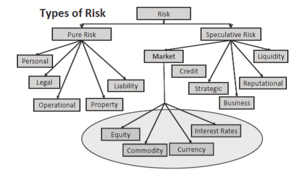
Risk can be categorized as either pure or speculative ^{[5] [6]} , as depicted in Figure 1. Regarding pure risk, there is no benefit or gain pertained to it, thus loss is the only possible outcome e.g. companies exposed to fraud or damage of assets etc. On the other hand, speculative risk can result into an uncertain degree of loss or gain e.g. a company can either gain or lose on investing in a new product, since there is a risk of market rejection. In this article emphasis is laid on speculative risk.

Risk Management

When dealing with project, program or portfolio management it is crucial to understand that a lot of uncertainties (risks) are pertained to them, since their eventual benefits are projected into the future (vision/goal). These uncertainties occur randomly within the lifecycle of the different categorize of management, thus eventually resulting into delays, budget overruns and eventually terminations, if not managed hence the importance of risk management.

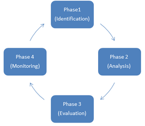
According to ISO 31000 ^[7] risk management is the coordination of activities to direct and control an organization with regards to risk. In literature^{[8] [9]} risk management can be decomposed into four continuous phases i.e. risk - Identification, Analysis, Evaluation and Monitoring as depicted in Figure 2 and elaborated below. Before embarking on a risk management course, it is crucial to commence with a risk management plan. Risk management planning is the structuring and detailing of how the risk management process is going to be conducted throughout the lifecycle of a project ^[10]. Subjects such as methodology, practices, roles and responsibilities, sequence and timing of activities are pertained to risk management planning ^[11].

• Phase 1: Risk Identification :

This phase involves the pinpointing of potential risks that might eventually affect a particular project in context and their causes. It is usually conducted by domain experts by means of brain storming^[12]

• Phase 2: Risk Analysis:

This phase involves the comprehension of the nature of the initially identified risks and an estimation of their consequences ^[13], since risk have different severity degrees. Risk analysis can be sub divided into qualitative and quantitative risk analysis. Both approaches can be utilized in one project but in order to conduct a quantitative analysis, estimates from the qualitative analysis is needed. On the other hand risk analysts can chose to stop with a qualitative risk analysis if the project is not too big.

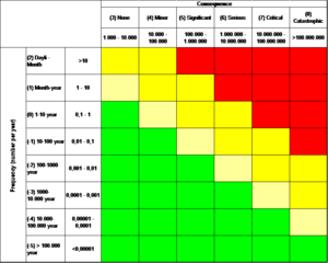
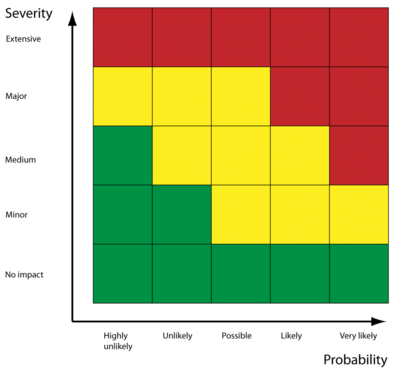
Qualitative risk analysis:In a qualitative risk analysis descriptions and estimates (mostly in monetary terms) of the different consequences pertained to the different risks, estimates of their occurrence (frequency) and means by which they can be mitigated are listed. Furthermore the different risks are prioritized, which provides the foundation for the evaluation phase. Figure 3 shows an overview of how the different risks can be prioritized according to severity.

Quantitative risk analysis:Quantitative risk analysis is a process of quantifying various impacts of identified risks imposed on a specific project in context, by means of using their estimates from the qualitative analysis. The quantification process is conducted by allocating different probability distributions to respective risks and thus simulating hypothetical events (scenarios) of the identified risks^[14]

• Phase 3: Risk Evaluation:

This phase involves the evaluation of the different risks by means of comparison in terms of severities and frequencies thus the establishment of tolerability levels. Organizations can in this phase chose to accept, try to avoid, transfer the risks or terminate the project if the risks are too high.

• Phase 4:Risk Monitoring and Control :

This phase involves the continuous monitoring, supervising and controlling of the different identified risks ^[15] . New risks that were not initially identified could also surface along a projects lifecycle, thus the necessity of continuously reassessing and revaluating risks. Figure 4 depicts a more detailed process of Risk management.

.

Monte Carlo Simulation

In order to elaborate on what a Monte Carlo simulation is, the following terms must be understood in order to facilitate the comprehension of the concept of Monte Carlo simulation:

• Random variable (Stochastic variable):

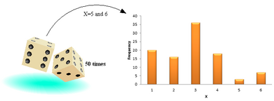
A variable is any defined characteristic that is subjected to variation either due to natural and /or imposed factors e.g. height, age, temperature etc. A random variable on the other hand is any function that allocates a numerical value to each possible outcome^[17] i.e. a measurement or a count of a variable (characteristic) that varies randomly according to a certain pattern. Random variables can be categorized into two categories depending on the type of outcome from a certain pattern; Discrete or continuous. Discrete random variables are outcomes of random variables that are either finite or countably infinite, whereas if the set of possible outcomes of a random variable is an interval, then it is continuous ^{[18] [19]} . E.g. when throwing two deices fifty times simultaneously as depicted in Figure 5, a player can’t predict what the outcome will be due to uncertainty, therefore when the outcome results into 5 and 6, the values are termed as random variables.

.

• Probability distribution:

Probability is the chance of something in particular occurring e.g. when playing Russian roulette with a six chamber revolver loaded with one bullet, the probability of pulling the trigger thus igniting the bullet is P(X=bullet)=1/6. A distribution on the other hand is the listing of viable/intervals of values of a characteristic (variable). A probability distribution can thus be defined as the probability structure of a random variable ^[20] i.e. in other words the probability (chance) of a random variable taking on a value within a certain set of possible outcomes, whereas each of those outcomes have a certain probability of occurring. It should be noted that when dealing with discrete random variables, the probability distribution of the variable is referred to as the probability mass function, and on the other hand probability density function when dealing with continuous random variables ^[21] .

Thus a Monte Carlo simulation can be defined as a quantitative approach of quantifying risks, by means of utilizing a probability distribution ^[22]. This is because risk is random and uncertain; therefore it can be classified as a random variable i.e. something that occurs by chance. Hence a Monte Carlo simulation of a particular project in context selects random variables from a given probability distribution of risk that is modeled by means of estimates. This is in order to figure out which risk has the highest certainty of occurring based on the probability distribution allocated to it. Furthermore, a Monte Carlo simulation enables the correlation of various risk factors, by means of incorporating a probability distribution for each conditional relationship^[23][24]. This thus facilitates the process of comprehending and assessing the various impacts of risks associated to a certain project and the pinpointing of ways in which they relate to each other.

Methodology

A probability distribution model of identified risks are attained by means of acquiring historic or domain expert data (elaborated below) and thus conducting a data fitting, to observe which distribution model suits the various identified risks the most. A Monte Carlo simulation utilizes the probability distribution by means of selecting random variables (represents various risks) within a defined range of parameters. The process of selecting random variables is performed with multiple iterations to simulate different possible outcomes in order to find the risk with the highest certainty of occurring. For the sake of simplifying and exemplifying; think of a company that is about to initiate a new project, the project group conducts a risk analysis thus identifying six risks that could affect their project during the qualitative risk analysis. The identified risks along with their estimates are then entered into a Monti Carlo simulation which then processes the data provided. An analogy in this case with regards to the Monti Carlo simulation is continuously throwing a six sided dice marked with R1, R2….. R6 (represents the identified risks) e.g. up to a thousand times and thus recording the frequencies at which they occur. All the six identified risk have an equal chance of occurring in this scenario i.e. 1/6 thus making the distribution to be applied, a uniform distribution, which is elaborated in the Data fitting section. This is a good way of understanding how a Monti Carlo simulation functions since it selects random variables from a given distribution and records the frequencies at which they occur. This iteration is done a couple of times to find the most likely risks. In order to conduct a Monti Carlo simulation of a given project, the following phases need to be undertaken:

Data sourcing

It is crucial to attain applicable data when working with a Monte Carlo simulation. This is in order to grasp vital information embedded in the final results. The more precise the data inputs are, the more valuable data can be extracted. In other words trash in equals to trash out. When dealing with data sourcing for a Monte Carlo simulation regarding risk, there are two forms of data that could be applied i.e. historic data (available) or domain expert knowledge (input from qualified experts)^[25]. A very good ex. of where domain expert knowledge is applied when conducting a risk analysis is within the construction industry. Experts that have worked within the field for years, thus acquiring knowledge and experience, use their foundation as a source for establishing estimates of price and time pertained to a certain building project. Historic data on the other hand can be sales data, cost of similar projects from the past or data from historic events etc.

Data fitting

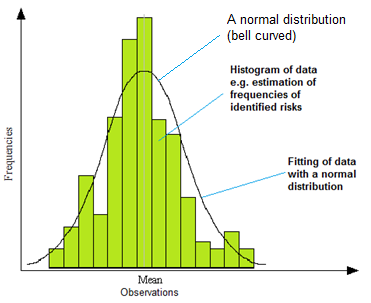
Data fitting is the process of identifying the most appropriate probability distribution to simulate observed (historic) or defined (domain expert) data. E.g. by plotting a histogram over observed data and then plotting a distribution over it (normal distribution) as depicted in Figure 4 1 to visually inspect if the distribution fits. In many cases it can be very difficult to pinpoint the exact distribution to apply, when there is more than one distribution that can fit. Thus the necessity of goodness of fit, whereby the Chi-squared and Kolmogorov-Smirnoff test can be applied to test how good a distribution fits to a set of observed data (Gupta, 2013) Common distributions applied in the simulation of risks in a Monti Carlo simulation are elaborated as follows:

• Normal Distribution:

When utilizing the normal distribution two parameters must be defined, i.e. the mean (average of the data set) and the standard deviation (the difference between the various random variables from the mean). It is an unbounded distribution i.e. the possible outcomes of the random variables covers all possible values. The values centered about the middle (mean) of the distribution are most likely to occur with a probability of 68 % i.e. with one standard deviation from the mean. This can be seen in Figure 6, where the random variables around the mean have the highest frequencies. The normal distribution can be utilized to simulate risk of inflation by means of historic data thus mitigating the risk of budget overruns.

.

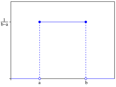
• Uniform Distribution:

In this form of distribution all variables have an equal chance of occurring as initially mentioned in the dice analogy example of a Monte Carlo simulation. Two parameters have to be defined when utilizing the uniform distribution i.e. the minimum and maximum values as depicted in Figure 7.

.

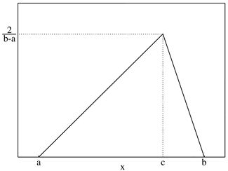
• Triangle Distribution:

This form of distribution is mostly applicable when dealing with domain expert data. When applying the triangle distribution three parameters have to be defined i.e. the minimum (optimistic), most likely (mode) and maximum (pessimistic) values^[26] as depicted in Figure 8. Triangle distributions are also bounded distributions since the possible outcomes of the random variables can only range within a defined interval

.

Iteration process

In this phase a Monte Carlo simulation software e.g. @Risk (works with excel), Latin hypercube, MATLAB etc. conducts a selecting process of random variables and identifies the most likely risks to occur based on the initially chosen probability distribution. Thereby simulating the likelihood of forecasted risks based on provided estimates.

Conclusion

Monte Carlo Simulations are utilized in facilitating the process of identifying the most likely risks to occur during a project which could obstruct progress, by means of quantifying them. This thus facilitates the process of understanding and evaluating risks. Monte Carlo simulations are particularly fruitful when dealing with large projects since different risks can be modeled and a distribution can also be used in defining how the different risks relate to each other thus making it more realistic. The advantages and disadvantages pertained to Monti Carlo Simulations are as follows:

Advantages

• Reduced cost, due to the enablement of quantifying and mitigation risk prior to the implementation of its respective project.
• Acquired results are probabilistic thus apart from showing what eventually could happen, it also shows the likelihood.
• Easier to estimate intervals than to a specific value.

Disadvantage

• A certain degree of uncertainty on forecasted models, due to assumptions of the future. i.e. projection into the future, where there is no data availability therefore having to settle with estimations
• If the probability distribution is not suitable for a particular risk simulation, the output will not be useful i.e. garbage in garbage out.

References

1. ↑ Gupta, Aparna,Risk Management and Simulation 2013
2. ↑ Hertz David B. & Thomas Howard,Risk analysis and its application 1983
3. ↑ WANG, Xing-xia; HUANG, Jian-wen,Risk analysis of construction schedule based on Monte Carlo simulation,International Symposium on Computer Network and Multimedia Technology (CNMT 2009)
4. ↑ Nemuth, Dr.-Ing. Tilo,Practical Use of Monte Carlo Simulation for Risk Management within the International Construction Industry,6th International Probabilistic Workshop 2008
5. ↑ Hertz David B. & Thomas Howard,Risk analysis and its application 1983
6. ↑ Gupta, Aparna,Risk Management and Simulation 2013
7. ↑ Danish Standards,ISO 31000 Risk management - Principles and guidelines 2009
8. ↑ Nemuth, Dr.-Ing. Tilo,Practical Use of Monte Carlo Simulation for Risk Management within the International Construction Industry,6th International Probabilistic Workshop 2008
9. ↑ Danish Standards,ISO 31000 Risk management - Principles and guidelines 2009
10. ↑ Tysiak, Wolfgang; Sereseanu, Alexander,International Journal of Computing 2010
11. ↑ Danish Standards,ISO 31000 Risk management - Principles and guidelines 2009
12. ↑ Tysiak, Wolfgang; Sereseanu, Alexander,International Journal of Computing 2010
13. ↑ Danish Standards,ISO 31000 Risk management - Principles and guidelines 2009
14. ↑ Suhobokov, Alexander; Application of Monte Carlo Simulation Methods in Risk Management,Journal of Business Economics and Management 2007
15. ↑ Danish Standards,ISO 31000 Risk management - Principles and guidelines 2009
16. ↑ Danish Standards,ISO 31000 Risk management - Principles and guidelines 2009
17. ↑ Johnson, Richard A; Freund, John; Miller, Irwin,Probability and Statistics for Engineers 2011
18. ↑ Montgomery, Douglas c,Design and Analysis of Experiments 2012
19. ↑ Johnson, Richard A; Freund, John; Miller, Irwin,Probability and Statistics for Engineers 2011
20. ↑ Montgomery, Douglas c,Design and Analysis of Experiments 2012
21. ↑ Montgomery, Douglas c,Design and Analysis of Experiments 2012
22. ↑ Tysiak, Wolfgang; Sereseanu, Alexander,International Journal of Computing 2010
23. ↑ McCabe, Brenda,Monte carlo simulation for schedule risks, Winter Simulation Conference Proceedings, Volume 2 2003
24. ↑ Hargreaves, John,Quantitative Risk Assessment in ERM, Enterprise Risk Management 2011
25. ↑ McCabe, Brenda,Monte carlo simulation for schedule risks, Winter Simulation Conference Proceedings, Volume 2 2003
26. ↑ McCabe, Brenda,Monte carlo simulation for schedule risks, Winter Simulation Conference Proceedings, Volume 2 2003