Analytic Hierarchy Process
(→The Numerical Scale) |
(→Limitations) |
||
| Line 244: | Line 244: | ||
The scale debated is a very heated debate and no one solution is defined. Saaty's original 1 to 9 scale is currently the most adapted scale worldwide, while scientists argue that the scale choice rather should depend on the person and the decision problem at any given time.<ref name="Ishizaka"></ref> | The scale debated is a very heated debate and no one solution is defined. Saaty's original 1 to 9 scale is currently the most adapted scale worldwide, while scientists argue that the scale choice rather should depend on the person and the decision problem at any given time.<ref name="Ishizaka"></ref> | ||
| + | |||
| + | |||
| + | ====Considerations regarding the limitations==== | ||
| + | The highlighted limitations showcase the importance of calculating the Consistency factor and consider the Sensitivity Analysis carefully. Utilizing these steps, should help counteract the qualitative biases and scale rating biases when applying the tool. | ||
=='''Bibliography'''== | =='''Bibliography'''== | ||
'''References''' <references /> | '''References''' <references /> | ||
Revision as of 02:13, 26 February 2018
Contents
|
Abstract
This will be written in the end
Introduction
History
The Analytic hierarchy process is a multi-criteria decision making (MCDM) method utilized to analyse, solve and prioritize complex decision, by rating and comparing multiple criteria and scenarios against each other [1] .
It was Thomas Saaty, regarded as one of the pioneers of Operations research which developed the Analytic Hierarchy Process throughout the 1970s. In the late 1960's, Saaty was recruited by the Arms Control and Disarmament Agency at the U.S. Department of state to direct their research projects. During his period there, he observed considerable communication difficulties between the scientists and lawyers at the department, both groups being the main contributors and decision makers in the project, which led to poor project results. Based on his experience from this period, Saaty was driven to develop a simple way to help ordinary people communicate better and make complex decisions, eventually resulting in the Analytic Hierarchy Process. From that day on, the Analytic Hierarchy Process has perhaps become the most widely used decision making method in the world with actual relevant applications counting in the thousands [2].
Application of the Analytic Hierarchy Process
Decision making and doing them right is one of the largest challenges that organizations have to face. This is especially true in the current competitive turbulent environment that organizations find themselves in. Decision making often involves multiple stakeholders throughout the organization with multiple different objectives. It has therefor become a critical factor for organization to make the right choices based on adequate and aligned objectives. This can be very hard as stakeholders tend to be subjective towards there own bias where they always choose the best alternative among those open to them, as they see them rather than focusing on the whole organizational perspective [3]. Humans tend to seek and interpret evidence in ways that will confirm there existing beliefs and hypothesis, well known in psychology as confirmation bias and thereby affecting multi-stakeholder decision making in organizational purposes[4].
The Analytic Hierarchy Process, as defined by Thomas Saaty, has been acknowledged for combining psychology and mathematics well to apply towards complex organizational decision making. The Analytic Hierarchy Process compares criteria, or alternatives with respect to a criterion in a pairwise manner. Each criteria and alternative is evaluated, based on a predetermined scale which has shown to capture individual preferences with respect to quantitative and qualitative attributes. The scale helps converts the evaluations to numerical values which are than utilized to calculate overall ratings for the possible alternatives and find the optimal solution [2]. As the qualitative input and the interpretation of the quantitative evaluations for the ratings can be inconsistent, the Analytic Hierarchy Process considers and calculates a consistency ratio for the ratings given, to prevent previously mentioned biases and to secure consistency throughout the ratings [5].
Considering how effective the Analytic Hierarchy Process is for complex decision making, it is often utilized by the PPM (Project Portfolio Management) for the prioritization and selection of projects in a portfolio. The selection of projects is often driver by multiple drivers and affected by multiple stakeholders. The Analytic Hierarchy Process , its application and overall understanding can therefor be considered very relevant for Project Portfolio Managers and Project Managers alike [6].
Methodology - A Step-By-Step approach
In the following section the Analytic Hierarchy Process and its application towards decision making is described in a step-by-step manner. Additionally, for a better understanding of the Analytical Hierarchy Process anexample has been made to showcase the practical usage of the tool, highlighted after every described step. The example is derived from the theory, but created by the author of the article and based on a fictional case. The case example is to consider improved scenarios for the medicinal distribution within a hospital, with pre-defined criteria and possible solution alternatives.
Define the Problem
The decision making should be driven by a stated problem. The problem should be well defined and the objectives of the problem should be broadened to consider all actors, objectives and possible outcomes. All criteria that influence the solution, the chosen outcome, are then to be identified[7].
Example: Background and Definition of the problem
A consultant team has proposed two new solutions to improve the efficiency, quality and cost of distributing medicine towards the patients within a hospital. The hospital has a low level of technology, minimal usage of IT systems and the medicinal storage is spread out throughout the hospital.
- The first solution proposes to implement a new IT solution, a so called ERP system, for improved quality and management of medicine. It is considered relatively investment light and easy to implement, but with low cost improvements. This solution will be referred to as the New ERP System solution.
- The second solution proposes to radically change the storage solutions within the hospital. All storage units are to be combined in one large stocking area, with improved distribution combined with smaller stock supermarket solutions and distribution medicinal runners, which fill up the supermarkets daily. An all new ERP solution is proposed as a part of the solution. This solution has been simulated and showcases improved cost, efficiency and quality of distribution. It does though need considerable investment and it is harder to implement.
The two scenarios are to be proposed towards a steering committee within the hospital, which will have to decide what they want to do. The current state is also an option. The steering committee will use the Analytical Hierarchy Process (AHP) method to decide between the solutions.
The consultant team has proposed the following criteria that have to be considered when choosing a future solution:
- A. Quality (quality of medicine distribution towards patience)
- B. Ease of Implementation (Easiness of implementing new solution)
- C. Investment (Cost of initial Investment)
- D. Direct Cost (Reduced cost of operations)
- E. Technology Usage (State of the art technology usage)
- F. Stock Availability (Transparency of stock availability)
- G. Efficiency (Efficiency in terms of daily operations)
Define the Problem Hierarchy
The factors which effect the final decision are then arranged in an hierarchic structure. This serves two purposes:
- It helps to structure the problem and thereby better understand the complex relations between all considered factors.
- It helps the decision maker to visually assess whether the issues stated in each level in the hierarchy are at the same level of importance and magnitude. This is important so factors can be considered accurately and of similar manner.
The hierarchy is sorted from the overarching goal at the top, to criteria and eventual sub-criteria, and then lastly the possible alternatives that are to be considered. [5]
Example: Define the Problem Hierarchy
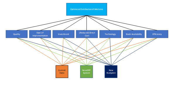
To start the process, the steering committee defines the hierarchy for the problem. The Distribution of medicine is defined as the overarching Goal, the pre-defined criteria shown below and lastly the three available solutions are defined as the alternatives. Each alternative has to consider each criteria in the hierarchy level above. The hierarchy is shown in figure xx.
Pairwise comparison and Calculate the Goal Priority
Next step is the Pairwise comparison of attributes on each level defined with a numerical rating, based on a pre-defined numerical scale by Saaty [5]. Comparison matrices are constructed for each set of pairwise comparisons. This requires n(n-1)/2 comparisons, n defined as the number of attributes in consideration on each hierarchy level. The rating scale for the pairwise comparison goes from 1 to 9, where if attribute A is of equal importance to attribute B, it receives a rating of 1. If attribute A is of absolute more importance than B, it receives a rating of 9. Likewise, if attribute A is considered absolutely more important than B, than attribute B should be rated with the reciprocal rating of A.
Based on the comparison matrices for each set, the priorities are obtained and utilized to weigh the priorities in the level below in the hierarchy.
Example: The Pairwise Comparison and Goal Priority
With the hierarchy in place, the weight of each criteria is considered. Each criteria is compared in a pairwise comparison utilizing The Fundamental Scale for Pairwise Comparisons, shown in figure x:
The comparison is done in a reciprocal matrix, with the size n x n. As there are 7 criteria, the matrix has to consider 49 values. The rating scale value is inserted for each pair comparison, read as row compared to column.
The Steering committee discusses each pair comparison and eventually comes to a conclusion, resulting in the table shown below:
To calculate the priority weight of each criteria, the table has to be normalized. This is done by dividing each rating with the sum of the given column. An example is the row criteria Technology Usage for column criteria Quality. This value is calculated as follows:
This is calculated for all values in the table and results in the following, as shown below:
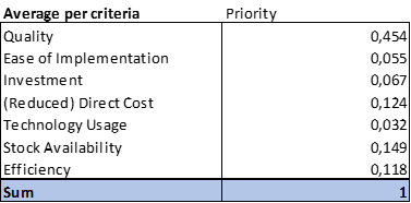
Lastly, to define the overall priority rating for each criteria, the average is calculated for each row criteria. This results in the following table:
Example: Ratings per Alternatives
With the criteria in place, the solution alternatives have to be compared pairwise as well and rated. The procedure is similar, where each alternative pair is considered for each criteria.
An example for the first step of the Quality Criteria is showcased as follows:
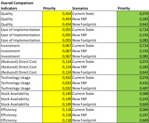
This is done for all 7 criteria and as before the table is then normalized. With all alternative pair-wize comparisons in place, the overall priority ratings per criteria for each alternative is shown in the table, figure xx, highlighted in green:
As shown in the table, column highlighted in yellow, the Quality criteria is considered to have the highest priority while the Technology Usage criteria is considered to be of the lowest importance
Consider how consistent the ratings are
After obtaining the priorities towards the hierarchy goal, it is important to consider how reliable the ratings are. As previously mentioned, the ratings are a pairwise comparison and can be subjectively bias, as they are based on individual or group perspectives towards each criteria. In psychology subjective bias is typically defined as Confirmation Bias, generally defined as the interpretation of evidence which is partial to ones existing beliefs and expectations. This bias can affect the overall solution, with certain criteria or alternatives weighing to much and thereby affecting the rating consistency [4].
To address this, a consistency ratio is calculated utilizing a framework and a consistency index (CI) put forward by Saaty (1997). [1]. A Principal Eigen Value is calculated, based on the global priority for each attribute. The sum of the Principal Eigen Values for all attributes are accumulated and divided with n, the number of attributes in the given hierarchy level. This gives a certain Inconsistency level. This Inconsistency level is then compared to the Consistency Index as proposed by Saaty, which is defined for each matrix of size n. The numerical value for each matrix of size n in the Consistency Index, has been calculated based on large samples of random matrices and the consistency indices of those matrices [7]. A Consistency Ratio is calculated, by dividing the Inconsistency level with the appropriate Consistency Index. If the Consistency Ratio is less than 0.1 (10%) than the matrix can be considered as being consistent. If it is higher than 10% it is advised to reconsider the attribute rating to achieve consistent measures [1].
Example: Consistency in criteria Ratings
To make sure that the steering committee was consistent throughout their criteria weight ratings, the Consistency Ratio has to be calculated. The Consistency Ratio (CR) is calculated by dividing the Inconsistency Ratio (IR) with the Consistency Index (CI) which is pre-defined for each matrix of the size n as explained in the step-by-step segment above.
First, the Principal Eigen Vector is needed. The Principal Eigen Vector is calculated by multiplying the overall priority rating for each criteria with the sum of rating for each attribute column. An example is the Principal Eigen Vector calculation for the Quality criteria. The row Quality criteria value of 0,454 is multiplied by the Quality' criteria column sum of 2,03 (as shown in figure xx). This calculates to:
The Principal Eigen Vector is calculated for all criteria and shown as follows:
Next the Inconsistency Ratio is calculated. The Inconsistency Ratio is based on the sum of all Principal Eigen Vectors and the amount of attributes. The amount of attributes are defined as n, and the sum of the Principal Eigen Vectors as z. The formula to calculate the Inconsistency ratio is as follows:
As there are 7 criteria (attributes), n is equal to 7. As shown in figure xx, the sum of the Principal Eigen Vectors is z = 7,558. Based on the formula, this gives:
The Consistency Index is based on the amount of attributes n, defined in the following table:
Again, as there are 7 criteria (attributes), n is equal to 7. Based on the table, that gives a Consistency Index (CI) of 1,32.
The Consistency Ratio is then calculated as follows:
This gives:
As the Consistency Ratio falls under 10%, the criteria ratings are considered to be consistent throughout the Matrix. The same calculations are repeated for the alternative ratings, which are also considered to be consistent as they likewise fall under 10%.
Overall weight of alternatives and optimal solution
After having considered the consistency and obtaining all the weighted priorities of criteria and alternative, it is possible to calculate the optimal alternative towards the overarching goal. This is done by calculatingthe weighted value per alternative and prioritizing the highest value.
Example: Overall weight of alternatives
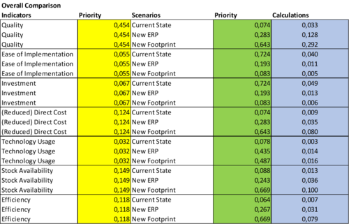
The weight for each alternative within each criteria is calculated by multiplying the priorities with each other. An example is when calculating the Quality priority value with the Current State priority value, as shown in figure xx below:
This is done for all criteria and the results are highlighted in blue, in the following table:
These priorities are than summed up an a matrix, where the sum of all criteria per alternative is calculated. The sum is the overall priority goal for the Optimized Distribution of Medicine, per alternative. The Goal priorities are shown in the following table, highlighted in gray:
As can be seen in the table, the New Footprint alternative is prioritized as the best solution with a Goal priority of 0.42 , based on all criteria and inputs for an optimized distribution of medicine within the hospital.
Perform a Sensitivity Analysis
Lastly, it is advised to perform a sensitivity analysis to observe the impact of modifying the input data towards the results. This is done by modifying the ranking of individual criteria as well the criteria weight towards the possible alternatives. If the global priority rank does not change, the results are considered to be robust. [1].
Example: Sensitivity Analysis
The consultant team proposes that a simple sensitivity analysis should be made. The steering committee wants to consider if they weighed the Quality criteria to high compared to the Investment criteria. They have therefor increased the weight of the investment by 0.3 and decreased the weight of the quality criteria by 0.3, as shown in figure xx:
When calculated through, this results in the following:
As can be seen for the overall goal priority, the New Footprint solution is still considered to be the optimal solution, with a Goal priority of 0.59 .
The Steering Committee and the consultant team feel confident in their consistent choices and rating considerations, and it is decided to go forward with the larger investment of an improved distribution footprint within the hospital.
Mathematical Background
Note: Consider to include explanation of the theoretical Mathematical Background
Application Areas
The Analytical Hierarchy Process is possible the most widely utilized decision making method in the whole world. There are more than a 1000 articles regarding the method and over a 100 doctoral dissertations. [2]
The method has been used in a wide spread of areas within both the public and the private sector. The main but not only examples of applications are as follows:
- Choices involving the selection of alternatives from a set of alternatives, as exemplified in the step-by-step segment above. This can be choosing a new technological solution, choosing a new supplier or deciding on a new product for a new market etc.
- Prioritization or evaluation of alternatives. Rather than only choosing one alternative, a few alternatives can be highlighted as the best ones. This could be relevant, for example if a company wants to consider a combination of alternatives.
- Resource allocation, for example budgeting for an array of multiple projects and defining which projects to prioritize and invest in. This application could be defined as a typical Project Portfolio Management approach, for defining projects to invest in within the portfolio.[2]
Limitations
Even though the Analytic Hierarchy Process is widespread and often defined as one of the most adapted decision tool in the world, there are limitations that have to be considered.
Pairwise Comparison
Due to the fact that all attributes on each level in the hierarchy have to be pairwise compared, the procedure can be quite cumbersome. This increases the resource and time usage needed to be able to define the optimal solution. Additionally, the pairwise comparison is very qualitative where participants evaluate the ratings based on individual or group input, which can be hard to quantify. This also includes quantitative information, as that has to be converted into the defined numerical scale.
The Numerical Scale
There have been some discussions regarding the pre-defined linear scale ranging from 1 to 9 and if it is the optimal scale for solutions. Many different versions of the scale have been proposed, which include among others:
- Geometric scale (9 values, ranging 1, 2, 4, 8, 16, 32, 64, 128, 256)
- Logarithmic scale (9 values, ranging logarithmically from 1 to 3,32)
- Balanced Scale (9 values, with a balanced weighted value approach from 1 to 9)
The scale debated is a very heated debate and no one solution is defined. Saaty's original 1 to 9 scale is currently the most adapted scale worldwide, while scientists argue that the scale choice rather should depend on the person and the decision problem at any given time.[1]
Considerations regarding the limitations
The highlighted limitations showcase the importance of calculating the Consistency factor and consider the Sensitivity Analysis carefully. Utilizing these steps, should help counteract the qualitative biases and scale rating biases when applying the tool.
Bibliography
References- ↑ 1.0 1.1 1.2 1.3 1.4 (“Ishizaka Alessio, Labib Ashraf, Analytic Hierarchy Process and Expert Choice: Benefits and Limitations, ORInsight, 22(4), p. 201–220, 2009)
- ↑ 2.0 2.1 2.2 2.3 (Forman Ernest H., Gass Saul I.,The Analytic Hierarchy Process - An Exposition, 2001)
- ↑ (Edwards Ward,The Theory of Decision Making, 1954)
- ↑ 4.0 4.1 (Nickerson Raymond S., Confirmation Bias: A Ubiquitous Phenomenon in Many Guises, 1998)
- ↑ 5.0 5.1 5.2 (Saaty Thomas L., Decision making with the analytic hierarchy process,Int. J. Services Sciences Vol. 1 No.1, 2008)
- ↑ (Vargas R. V., Using the analytic hierarchy process (ahp) to select and prioritize projects in a portfolio, 2010
- ↑ 7.0 7.1 (Vaidy Omkarprasad S., Kumar Sushil, Analytic hierarchy Process: An overview of applications, European Journal of Operational Research 169, 2006)


