Test15

Decision making is one of the most important tasks in the management process and it is often a very difficult one. When having knowledge regarding the states of nature, subjective probability estimates for the occurrence of each state can be assigned. In such cases, the problem is classified as decision making under risk . In the decision making process, all relevant information is evaluated through decision analysis (DA). The decision analysis process consists of the use of a decision tool and a decision theory. The decision tree is the most commonly applied decision tool in the decision analysis . The decision theory of interest in the decision analysis, regarding the decision making under risk, is the expected value of criterion also referred to as the Bayesian principle. This is the only one of the four decision methods that incorporates the probabilities of the states of nature .

---

Methologdy

Risk analysis and risk management is an important tool in the construction management process. Risk implies a degree of uncertainty and an inability to fully control the outcomes or consequences of such an action. The objective of a decision analysis is to discover the most advantageous alternative under the circumstances .

Decision analysis is a management technique for analyzing management decisions under conditions of uncertainty . The decision problems can be represented using different statistical tools applied to the mathematical models of real-world problems. An important and relevant decision tool to represent a decision problem is a decision trees. A decision tree is a graphical representation of the alternatives and possible solutions, also challenges and uncertainties. In decision analysis, formulating the decision problem in terms of a decision tree is a favorable visual and analytical support tool, where the expected values of competing alternatives are calculated.

Theory and principles

The following provides the theory and principles behind the decision making under risk, using Bayesian decision analysis. An overview of the principles and construction regarding the decision tree is provided as well as the decision theory regarding the decision tree analysis.

Decision tree

A decision tree (DT) is a chronological representation of the decision process. It is particularly suitable where a series of decisions are to be established and/or several outcomes appear at each stage of the decision -making process, it is therefore convenient in analyzing multi-stage decision processes. The number of alternative actions can be exceptionally large and an outline for the systematic analysis of the corresponding consequences is therefore expedient.

Decision trees is an effective decision tool in the decision-making, because it: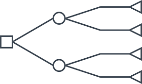

Figure 1: Decision tree diagram (click to zoom)

• Provides a clear overview of the situation so that all possibilities can be investigated

• Allows to fully analysis the potential consequences of a decision

• Provides an outline in which to compute the values of consequences and the probabilities of achieving them.

• Assists obtaining the best decisions based on existing information and best estimates.

A decision tree is a schematic, tree-shaped diagram representation of a problem and all possible courses of action in a particular situation and all possible outcomes for each possible course of action. The diagram is constructed of branches and each branch of the decision tree represents a possible decision, occurrence or reaction see figure 1. The tree is structured to show how and why one choice may lead to the next, with the use of the branches indicating each option is mutually exclusive.

A decision tree consists of three types of nodes:

• Decision (choice) Node

• Chance (event) Node

• Terminal (consequence) Node

There is no universal set of symbols applied when constructing a decision tree but the most common ones is a square to represent the decision node, a circle for the chance event and a triangle for the terminal node.

Construction of decision tree

For the purpose of illustrating the construction of a decision tree, the following considers a simple decision problem. An old bridge has been subject to deterioration, control data reveal that the bridge structure may be damaged. However, this cannot be indicated with certainty. If the bridge is damaged, it is unfit for service and a new one needs to be constructed. Your company is hired to find the best solution of two alternatives:

1. Alternative a₁: Do nothing
2. Alternative a₂: Repair the bridge

The decision-making process involves evaluating weather is more beneficial to do nothing or repair the bridge, the alternative associated with the lowest risk is in this case the alternative with the lowest expected cost.

Figure 2: Decision tree (click to zoom)

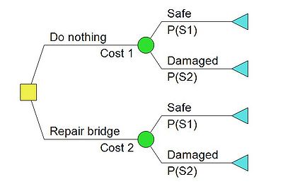
Figure 2 illustrates the constructed decision tree related to the provided example. The diagrams are created by the author using the program ‘'DPL9'’ which is decision tree-based, decision analytic software tool, developed by Syncopation Software . The tree is constructed from right to left in following three steps:

1. The first node drawn is the decision node, a branch emanating from a decision node corresponds to a decision alternative, which in this case are either to repair the bridge or do nothing. It includes a cost or benefit value, which in this example is referred to as cost 1 and cost 2. The decision node is displayed as a yellow square.


2. The next node is the chance node, since either of the alternatives does not lead to a new the decision. A branch emanating from a state of nature node (chance node) corresponds to a particular state of nature, and includes the probability of this state of nature. For both alternatives the branches has the same outcome, either the bridge is safe and fit for service or the bridge is damaged and a new needs to be constructed. The probability associated with the bridge being safe or damaged, are denoted P(S1) and P(S2), respectively. The chance node is illustrated whit a green circle.


3. The final node is the terminal node, this represent the cost consequence related to the choice of decision branch for all possible outcomes. The value of the each terminal node, are the total sum of the cost related to each branches. This value is also called the net path value (NPV). The terminal node is presented by the use of a blue triangle.

Decision theory

Decision theory is an analytical and systematic approach to tackle problems. Decision theory is the part of probability theory that is quantifying the consequences of uncertain decisions. This can be applied to state the objectivity of a choice and to optimize decisions .

The decision method applied in decision making under risk, is the expected value of criterion, because it incorporates the probabilities of the states of nature. The expected value of criterion contains the analysis of the expected monetary value (EMV), or simply expected value, which is the foundational concept on which decision tree analysis is based. EMV is a tool and technique, a numerically analyze performed concerning the influence of identified risks on overall project objectives. The EMV of risk is:

Expected Monetary Value= Probability of the Risk x Impact of the Risk.

EMV computes the average outcome when the future contains uncertain situations; it is the sum of the different scenarios connected to the chance node. The decision made at the decision nodes is therefore based on the expected monetary values of the related alternatives. Depending on the state of information regarding the probability at the time of the decision analysis, three different analysis types are distinguished, namely prior analysis, posterior analysis and pre-posterior analysis . Each one of these is important in practical applications of decision analysis and the basic theory is therefore outlined briefly in the following, with the utility represented in the simplified manner through costs.

Prior analysis

The prior analysis is a decision analysis performed with known information. The prior probability is the unconditional probability used in the analysis to quantify the beliefs before any evidence is taking into account. This state is often referred to as the state of nature and can be indicated by $\scriptstyle \theta$ . The probabilistic description $\scriptstyle P[\theta]$ of the state of nature is usually called a ‘’prior description’’ and expressed as $\scriptstyle P'[\theta]$ .

When the probabilities of the various state of nature corresponding to different consequences have been estimated, and the consequences for the final outcome determined, the analysis consists of the calculation of the expected utilities corresponding to the different action alternatives. The optimal decision is identified as the expected cost and presented as $\scriptstyle E'[C]$ when the decision is based on the prior information. The expected cost is equal to the expected monetary value of the action alternative corresponding to the largest expected utility.

Posterior analysis

The posterior analysis is the conditional probability that is assigned when additional information becomes available. The conditional probabilities form the basis of updating of probability estimates based on new information, knowledge or evidence, which makes conditional probabilities of interest in risk and reliability analysis. The conditional probability is the probability of an event, given that another event has already accord. The posterior probability of an event $\scriptstyle \theta_i$ , given that another event $\scriptstyle A$ has occurred is therefore expressed as:

${P''[\theta_i | A] = \frac {P[A|\theta_i] P' [\theta_i]} {P'[A]}}$

The conditional term $\scriptstyle{P'[A|\theta_i]},$ can be referred to as the likelihood, the probability of observing a definite state given the true state. The term $\scriptstyle{P'[\theta_i]},$ is the prior probability of the event $\scriptstyle \theta_i$, so the unconditional probability before any information about the event $\scriptstyle A$. $\scriptstyle{P'[A]},$ is the probability of the event $\scriptstyle A$ and can be written as:

${P'[A]=\sum_{i=1}^n P[A|\theta_i] P' [\theta_i]}$

Having determined the updated probabilities, the probabilities are assigned the different actions. When the posterior probabilities are know, it is possible to quantify the expected values. The expected cost related to the posterior analysis is denoted $\scriptstyle E''[C|A]$. The notation show that the value of the expected cost is based upon conditional probability, meaning that the result of the expected cost is when event $\scriptstyle A$ has occurred.

Pre-posterior Analysis

The objective of pre-posterior analysis is to determine whether the value of the prediction is greater or less than the cost of the information. ‘’Posterior’’ refers to the revision of the probabilities and the ‘’pre’’ indicates that this calculation is performed before paying the fee. The goal is therefore to choose the experiment or experimental design whit largest utility . The pre-posterior analysis involves the determination of the conditional, posterior probability. While the posterior analysis is based on the fact that event $\scriptstyle A$ has occurred the pre-posterior analysis, takes in the probability of the event $\scriptstyle A$ occurring. The expected cost $\scriptstyle E[C]$ based on the pre-posterior analysis is therefore expressed as:

${E[C]=\sum_{i=1}^n P'[A_i] E'' [C |A_i]}$

Where $\scriptstyle n$is the number of different possible experiment outcomes. The posterior expected cost $\scriptstyle {E'' [C |A_i]}$ for the different experiment outcomes, is therefore a process in preforming the pre-posterior analysis. The probability $\scriptstyle {P' [A_i]}$ is the prior probabilities of the different events.

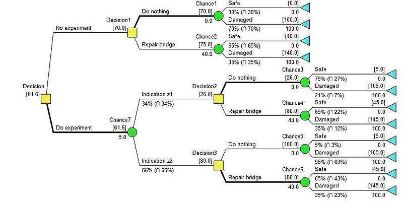
Bayesian decision analysis

The theory and principles of decision making under risk has been presented. The theory is applied to different examples. The data used in the examples is fictive and constructed by the author and is there for comparable to any true data. The scenarios in the examples is, however, situations that are representable for the decision making under risk when managing constructions.

Example 1 - Prior analysis

This example provides the decision analysis regarding the decision making under risk. The same scenario as represented previous under the construction of the decision tree is used. The two alternatives are either to do nothing or to repair the bridge. The following information is now provided:

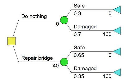
It is estimated that there is a 30% probability that the bridge structure is safe. If the bridge is repaired then the probability of the bridge structure having damaged is 35%. Table 1 provides the probabilities used in the construction of the decision tree in figure 3.

Table 1: Probabilities related to the two alternatives

	a1- Do nothing	a2- Repair bridge
$\scriptstyle P'[\theta_1]$ - Safe	0.30	0.65
$\scriptstyle P'[\theta_2]$ - Damaged	0.70	0.35

Figure 3: Decision tree example 1 - prior analysis (click to zoom)

It is seen that the probabilities are prior probabilities; therefore, a prior analysis is performed. If the bridge structure is damaged, then a new bridge is required which is associated with a cost of $100 mio. If the structure is safe then the cost is $0. The cost of repairing the bridge is $40 mio. The decision analysis can now be executed, starting out with the construction of the decision tree. The nodes and branches of the decision tree for this situation are already shown in figure 2, the missing costs and probabilities are assigned in figure 3. The two alternatives are provided with the related costs, the branches alternating from the decision nodes is provided with the probabilities of state of nature, that are presented in table 1 and their associated expenses. The net pressure value is not represented at the terminal nodes in figure 3, which is due to the fact the decision tree is drawn in DPL9 the program is quantifying the values at the terminal nodes, when the decision analysis is performed. The branches therefore need to be provided with their individual, related values. For simplicity and understanding the net pressure values are shown in table 2.

Table 2: Net pressure values related to the two alternatives - example 1

	a1- Do nothing	a2- Repair bridge
NPV 1 - Safe	$0 mio.	$40 mio.
NPV 2 - Damaged	$100 mio.	$140 mio.

The next step in the decision analysis is to compute the expected monetary values; the calculations are done from left to right, starting with the chance nodes having branches associated with the terminal nodes.

1. chance node - associated with alternative a ₁

$\textstyle EVM_{a_1}=P'[\theta_1] \cdot NPV_1 + P'[\theta_2] \cdot NPV_2=0.3 \cdot $0 mio. + 0.7 \cdot $100 mio.=$70 mio.$

2. chance node - associated with alternative a ₂

$\textstyle EVM_{a_2}=P'[\theta_1] \cdot NPV_1 + P'[\theta_2] \cdot NPV_2= 0.65 \cdot $40 mio. + 0.35 \cdot $140 mio.=$75 mio.$

The expected monetary values at the chance nodes are now established. The expected cost at the decision nodes is based on the expected monetary value for the two alternatives. In this example the utility is represented in a simplified manner through the costs whereby the optimal decisions is identified as the decisions minimizing expected costs, which then is equivalent to maximizing expected utility. The expected cost based on the prior information is therefore:

$\textstyle E'[C]=min \{EVM_{a_1};EVM_{a_2} \}= min \{$70 mio.;$75 mio.\}=$70 mio.$

It is seen that action alternative a ₁ - Do nothing, yields the lowest expense, $\scriptstyle EVM_{a_1}$, meaning that this action alternative is the optimal decision, since it is associated with the largest expected utility.

Figure 4: Decision analysis example 1 - prior analysis (click to zoom)

Figure 4 show results of the decision analysis preformed in DPL9. In figure 4 the net path values are given at the terminal nodes, as well as the expected monetary values at the chance nodes and the expected cost. The branch emanating alternative a ₁ is bold, confirming decision way. The values established during the decision analysis process is shown brackets above the branches, while the input data is shown under the branches.

Example 2 - Posterior analysis

When additional information becomes available, the probability structure in the decision problem may be updated. The case presents how to comprehend decision analysis in situations with conditional probability. In this situation, same scenario and prior information presented in example 1, is observed. Knowledge about prior probability and cost can be obtained in table 1 and figure 3. More information is acquired through a study about the chances of a bridge repair. The study costs $10 mio. Table 3 contains the estimation of the success rate (structure safe) of the bridge repair in the study,

Table 3: Study indication of bridge repair success

	Bridge repair results
	Structure safe	Structure damaged
Indication I	0.75	0.25

Given the result of the study, the updated conditional probability or the posterior probability $\scriptstyle P''[\theta_i | I ]$ is evaluated by use of the Bayes' rule. The likelihood of the structure being safe $\scriptstyle P[I|\theta_1]=0.75$ and likelihood of the structure being damaged is $\scriptstyle P[I|\theta_2]=0.25$. The probability of the indication $\scriptstyle P'[I]$ is then:

$\textstyle {P'[I] = P[I|\theta_1] \cdot P'[\theta_1]+ P[I|\theta_2] \cdot P'[\theta_2]=0.75 \cdot 0.65 + 0.25 \cdot 0.35 =0.575}$

The posterior probabilities are then:

$\textstyle {P''[\theta_1 | I] = \frac {P[I|\theta_1] P' [\theta_1]} {P'[I]}}= \frac {0.75 \cdot 0.65} {0.575}=0.85$

$\textstyle {P''[\theta_2 | I] = \frac {P[I|\theta_2] P' [\theta_2]} {P'[I]}}= \frac {0.25 \cdot 0.25} {0.575}=0.15$

Figure 5: Decision tree example 2 - posterior analysis (click to zoom)

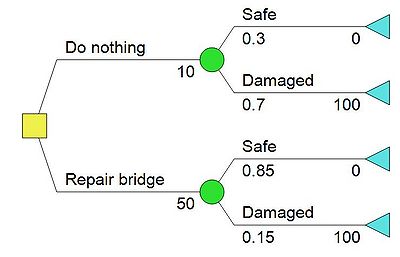
The expenses associated with the studies needs to be accounted for, which means that the cost related to alternative a ₁ is $10 mio., instead of the previous $0 mio. Alternative a ₂ is $50 mio. for the bridge repair including the study. The posterior probabilities regarding the bridge repair has been established and the computed decision tree is presented in figure 5. The structure of the decision tree has remained the same, howeever, the probabilites regarding the bridge repair and the costs related to chose of action is changes in comparison to the prior analysis in figure 3. The probabilities regarding alternative a ₁ remains the same unconditional, prior probabilities, hence the study is only related to the bridge repair. The net path values related to the terminal nodes are presented in table 4.

Table 4: Net pressure values example 2 - posterior analysis

	a1- Do nothing	a2- Repair bridge
NPV1	$10 mio.	$50 mio.
NPV2	$110 mio.	$150 mio.

Having determined the updated probabilities, the expected monetary values is then:

1. chance node - associated with alternative a ₁

$\textstyle EVM_{a_1}=P'[\theta_1] \cdot NPV_1 + P'[\theta_2] \cdot NPV_2=0.3 \cdot $10 mio. + 0.7 \cdot $110 mio.= $80 mio.$

2. chance node - associated with alternative a ₂

$\textstyle EVM_{a_2}=P''[\theta_1 | I] \cdot NPV_1 + P''[\theta_2 | I] \cdot NPV_2= 0.85 \cdot $50 mio. + 0.15 \cdot $150 mio. =$65 mio.$

The posterior expected cost $\scriptstyle E''[C|I]$ of the utility corresponding to the optimal action alternative is readily obtained as:

$\textstyle E''[C|I]=min \{EVM_{a_1};EVM_{a_2} \}=min \{$80 mio.;$65 mio. \}=$65 mio.$

Considering the additional information, it is seen that the optimal decision has been switched to action a ₂ as compared to the prior decision analysis. This will give the expected minimum cost $\textstyle E''[C|I]=65 mio.$.

Figure 6: Decision analysis example 2 - posterior analysis (click to zoom)

Figure 6 show results of the decision analysis preformed in DPL9. In figure 6 the net path values are given at the terminal nodes, as well as the expected values at the chance nodes. The branch representing alternative a ₂ , is bold, confirming the decision way.
¨

Example 3 - Pre-Posterior analysis

Often the decision maker has the possibility to ‘buy’ additional information through an experiment before making the choice of action. If the cost of this information is small in comparison to the potential value of the information, the decision maker should perform the experiment. If several different types of experiments are possible, the decision maker must choose the experiment yielding the overall largest expected value of utility. The conditional probability is used in the pre-posterior analysis. Let the prior condition be the same as the one presented in example 1. The alternative actions have however change, since there now is the option to install a SHM (Structural health monitoring) system. This gives the action alternatives no do the experiment $\scriptstyle {e_1}$ or do the experiment $\scriptstyle {e_2}$, before chosen between doing nothing or repair the bridge. The SHM system indicates either the structure is safe $\scriptstyle {z_1}$ or damaged $\scriptstyle {z_2}$. The cost of the SHM system is $5 mio. For to the finite precision, the system indications are probabilities depending the states. Table 5 present the indications of the SHM system.

Table 5: Structural health monitoring indications

Indication	$\scriptstyle \theta_1$	$\scriptstyle \theta_2$
z 1 - Safe	0.9	0.1
z 2-Damaged	0.1	0.9

The likelihood probabilities are presented in table 5, where $\scriptstyle P[z_1|\theta_1]=0.9$, $\scriptstyle P[z_1|\theta_2]=0.1$, $\scriptstyle P[z_2|\theta_1]=0.1$ and $\scriptstyle P[z_2|\theta_2]=0.9$. These are used in the calculations regarding the updated conditional probability or posterior probability. The probability of the indications $\scriptstyle {P'[z_1]}$ and $\scriptstyle {P'[z_2]}$

$\textstyle {P'[z_1] = P[z_1|\theta_1] \cdot P' [\theta_1]+ P[z_1|\theta_2] \cdot P' [\theta_2]=0.9 \cdot 0.3 + 0.1 \cdot 0.7 =0.34}$

$\textstyle {P'[z_2] = P[z_2|\theta_1] \cdot P' [\theta_1]+ P[z_2|\theta_2] \cdot P' [\theta_2]=0.1 \cdot 0.3 + 0.9 \cdot 0.7 =0.66}$

The posterior probabilities are then:

$\textstyle {P''[\theta_1 | z_1] = \frac {P[z_1|\theta_1] P' [\theta_1]} {P'[z_1]}}= \frac {0.9 \cdot 0.3} {0.34}=0.79$

$\textstyle {P''[\theta_2 | z_1] = \frac {P[z_1|\theta_2] P' [\theta_2]} {P'[z_1]}}= \frac {0.1 \cdot 0.7} {0.34}=0.21$

$\textstyle {P''[\theta_1 | z_2] = \frac {P[z_2|\theta_1] P' [\theta_1]} {P'[z_2]}}= \frac {0.1 \cdot 0.3} {0.66}=0.05$

$\textstyle {P''[\theta_2 | z_2] = \frac {P[z_2|\theta_2] P' [\theta_2]} {P'[z_2]}}= \frac {0.9 \cdot 0.7} {0.66}=0.95$

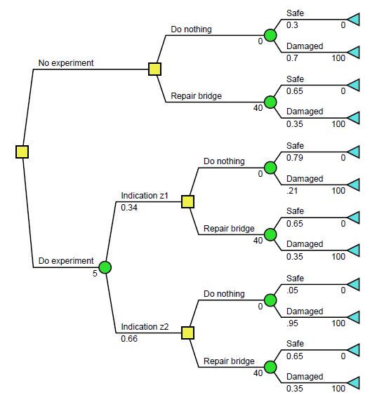
The construction of the decision tree is presented in figure 7. The structure of the diagram defers from the decision trees constructed in example 1, figure 3 and example 2, figure 5. The decision tree becomes larger, since the pre-posterior analysis consists or more possible outcomes and need to account for every possible scenario related to the option of weather install or not install the SHM system. The installment of the SHM system, does not have any influence on the probabilities related to the repair of bridge, opposite the scenario in example 2, where the study only had an influence on the bridge repair.

Figure 7: Decision tree example 3 - Pre-posterior analysis (click to zoom)

In comparison to figure 5 which represent the posterior probability, figure 7 also have the probabilities related to the indications included in the analysis and the prior state, since it evaluates weather or not to buy additional information. The net path values are found and presented in table 6.

Table 6: Net pressure values example 3 - pre-posterior analysis

	e1- No experiment		e2- Do experiment
			z1- Indication safe		z2- Indication damaged
	a1- Do nothing	a2- Repair bridge	a1- Do nothing	a2- Repair bridge	a1- Do nothing	a2- Repair bridge
NPV1	$0 mio.	$40 mio.	$5 mio.	$45 mio.	$5 mio.	$45 mio.
NPV2	$100 mio.	$140 mio.	$105 mio.	$145 mio.	$105 mio.	$145 mio.

When the probabilities and net path values is determined, the expected monetary values can then be quantified. First all the chance nodes to the right in figure 7 is investigated, hence all the chance nodes associated with terminal nodes. The expected monetary value for the six chance nodes is then:

1. chance node - associated with alternative e ₁ - a ₁

$\textstyle EVM_{e_{1}-a_1}=P'[\theta_1] \cdot NPV_1 + P'[\theta_2] \cdot NPV_2=0.3 \cdot $0 mio. + 0.7 \cdot $100 mio.= $70 mio.$

2. chance node - associated with alternative e ₁ - a ₂

$\textstyle EVM_{e_{1}-a_2}=P'[\theta_1] \cdot NPV_1 + P'[\theta_2] \cdot NPV_2=0.65 \cdot $40 mio. + 0.35 \cdot $140 mio.= $75 mio.$

3. chance node - associated with alternative e ₂ - z ₁ - a ₁

$\textstyle EVM_{e_{2}-z_1-a_1}=P''[\theta_1 | z_1] \cdot NPV_1 + P''[\theta_2 | z_1] \cdot NPV_2= 0.79 \cdot $5 mio. + 0.21 \cdot $105 mio. =$26 mio.$

4. chance node - associated with alternative e ₂ - z ₁ - a ₂

$\textstyle EVM_{e_{2}-z_1-a_2}=P'[\theta_1] \cdot NPV_1 + P'[\theta_2] \cdot NPV_2= 0.65 \cdot $45 mio. + 0.35 \cdot $145 mio. =$80 mio.$

5. chance node - associated with alternative e ₂ - z ₂ - a ₁

$\textstyle EVM_{e_{2}-z_2-a_1}=P''[\theta_1 | z_2] \cdot NPV_1 + P''[\theta_2 | z_2] \cdot NPV_2= 0.05 \cdot $5 mio. + 0.95 \cdot $105 mio. =$75 mio.$

6. chance node - associated with alternative e ₂ - z ₂ - a ₂

$\textstyle EVM_{e_{2}-z_2-a_2}=P'[\theta_1] \cdot NPV_1 + P'[\theta_2] \cdot NPV_2= 0.65 \cdot $45 mio. + 0.35 \cdot $145 mio. =$80 mio.$

The expected monetary values for the three decision nodes related to alternatives a₁ and a₂, is then established, the value is determined as the minimum cost, which is equivalent to the largest utility. The expected monetary values are then:

1. decision node - associated with alternative e₁

$\textstyle EVM_{e_1}=min \{ EVM_1; EVM_2\}= = $70 mio.$

2. decision node - associated with alternative e₂ - z₁

$\textstyle EVM_{e_2-z_1}=min \{ EVM_1; EVM_2\}=0.65 \cdot $40 mio. + 0.35 \cdot $140 mio.= $75 mio.$

3. decision node - associated with alternative e₂ - z₂

$\textstyle EVM_{e_2-z_2}=min \{ EVM_1; EVM_2\}=0.65 \cdot $40 mio. + 0.35 \cdot $140 mio.= $75 mio.$

The last expexted monetary value that needs to be evaluated is related to the last chance node. The chance node associated with the two indications z ₁ and z ₂ . The two quantified expected monetary values EVM and EVM together with the probabilitise P (z) and P(z) are therefore used, this gives:

'7. chance node - associated with alternative e ₂

The expected cost $\scriptstyle E[C]$ for the pre-posterior analysis is then found as:

$\textstyle E[C]=min \{EVM_{};EVM_{} \} = $70 mio.$

It is seen that the lowest expected cost, largest utility, is obtained by installing the strutural health monetering system. Figure 8 show the reults of the decision analysis preformed in DPL9. The figure show the net path values at the terminal nodes and the expected monetary values for both the chance and the decision nodes. The decision tree gives a convinenet overview of the paths and the related costs and probabilities. Example 3 gives a better presentation of the benefits regarding using a decsion tree, compared to the two previous examples.

Figure 8: Decision analysis example 3 - Pre-posterior analysis (click to zoom)

Annotated bibliography

Wu, G., Zhang, J. and Gonzalez, R. (2004) Decision Under Risk, in Blackwell Handbook of Judgment and Decision Making: This chapter of the handbook provides and introduction to decision making under risk, it present many phases in the history of risky decision-making research and highlight the differences and similarities between how economists and psychologists have approached this subject.

 (eds D. J. Koehler and N. Harvey), Blackwell Publishing Ltd, Malden, MA, USA. doi: 10.1002/9780470752937.ch2

Knight, F. H. (1921) Risk, Uncertainty, and Profit: This book presents the work of Frank Knight, a economist at University of Chicago, who distinguished risk and uncertainty. Knights point of view, was that an ever-changing world provides new opportunities for the industry to create profit, but also brings imperfect knowledge related to future events.

Karabadji, Nour El Islem et al. “An Evolutionary Scheme for Decision Tree Construction.” Knowledge-based Systems 119 (2017): 166–177. Web. (basis for decision tree)

R.C. Barros, A. de Carvalho, A.A. Freitas, Automatic Design of Decision-Tree

Induction Algorithms, SpringerBriefs in Computer Science, Springer International Publishing, New York City. URL https://books.google.co.kr/books? id¼PFqEBgAAQBAJ, 2015.

Delmar, M.V., and J.D. Sorensen. “Probabilistic Analysis in Management Decision Making.” Proceedings of the International Offshore Mechanics and Arctic Engineering Symposium 2 (1992): 273–282. Print.

Donegan, H. A. “Decision Analysis.” Sfpe Handbook of Fire Protection Engineering, Fifth Edition (2016): 3048–3072. Web.

Khalili Damghani, K., M. T. Taghavifard, and R. Tavakkoli Moghaddam. “Decision Making Under Uncertain and Risky Situations.” (2014): n. pag. Web.

Annotated:

Goodwin, Paul; Wright, George. (2004). Decision Analysis for Management Judgment. Wiley