Data-Driven Decision-Making under Uncertainty
Developed by Anton Reiling
There are several approaches to reach decisions under uncertainty under the assumption of reliable, fixed data. The degree of complexity and scope among the approaches differs considerably, which is why they should be selected according to the use case.
Starting with the simple approaches the Minimax and Maximax criterion consider the worst or best possible outcome of decision alternatives. The Hurwicz Criterion offers a mix between these two approaches depending on the predefined Optimism Parameter. The Minimax Regret Criterion considers the opportunity costs caused by choosing an alternative to reach a decision and the Laplace Criterion compares the expected values of the alternatives. However, due to simplifications and assumptions these methods are limited to rather simple problems with low complexity. This is because they lack the possiblity to assess risk, qualitative inputs and heterogenous probabilities for different outcomes.
For more complex problems, approaches like the Monte Carlo Simulation and Sensitivity Analysis can be used, while also requiring more effort to be conducted. However, they can also be used to support and analyze the classical approaches. In this article, the Laplace Criterion will be examined using a Monte Carlo Simulation and the critical Optimism Parameter of the Hurwicz Criterion is determined using a Sensitivity Analysis. There is also the concept of Robust Decision Making, which combines different tools to help to make better and more profound decisions.
All these approaches can be used within Project, Program and Portfolio Management, for example to compare two offers for Outsourcing Contracts within Project Management, which is illustrated later in this article. Depending on the decision-making approach different results will be yielded, which clarifies their respective focus and susceptibility to outliers.
Contents |
The Decision-Making Process

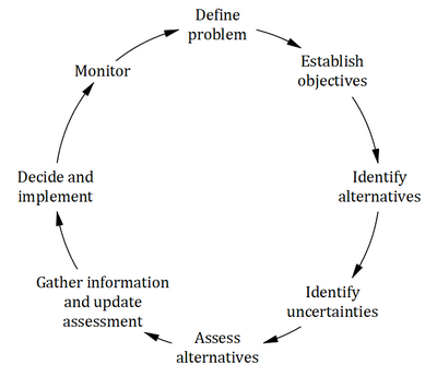
In order to reach a sensible decision for a specific problem, certain steps have to be followed:
- Step 1: Define the problem: Specify the problem framework with the respective requirements regarding costs, time horizon, etc. It is important to reflect, which criterion should exactly be examined. This could be the for example the cost, profit, payback or Return on Investment. If non-economic issues should be compared, methods to quantify those apects have to be used. [2]
- Step 2: Establish the objectives: Describe the objectives for the given problem to create a foundation to compare later alternatives on depending on their degree of fulfillment and performance.
- Step 3: Identify alternatives: Work out possible alternatives that can satisfy the objectives and narrow them down to a shortlist that can be examined under reasonable effort later.
- Step 4: Identify uncertainties: Elaborate possible scenarios that can inlfuence the utility or cost of alternatives and connect them to the alternatives with their respective values.
- Step 5: Assess alternatives: Conduct research or apply decision-making tools to find out, which alternative satisfies the given objectives best.
- Step 6: Gather information and update the assessment: Gather data to verify if the preferred alternative from step 5 is really the best alternative of all the available ones. In case crucial data was overlooked, repeat step 5.
- Step 7: Decide and implement: Make a final decision regarding which alternative to choose and assign tasks and responsibilities to it
- Step 8: Monitor: Continously track the progress of the implementation to be able to plan adjustments if necessary [1]
Within the scope of this article, steps 5, 6 and 7 will be examined in further detail.
Fundamental assumptions
Differences between Decision-Making under Uncertainty and Risk
While decison-making under risk implies a certain probability for each possible outcome, decision-making under uncertainty assumes that these probabilites are unknown and thus each scenario is considered equally important. This subsequently leads to a higher inaccuracy of uncertainty problems compared to risk problems. An example for that would be a problem with 3 possible outcomes: Best case, most probable case and worst case. While for decision-making under risk the both extreme scenarios would be considered with a presumable low probability and thus a low weight, for decision-making under uncertainty all of the outcomes would be regarded in the same way, which means that in this case outliers have a considerably higher impact to the decision. [3]
Decision-Making Approaches
There are various approaches that can be used for decision-making. In the following, the classical strategies will be presented, that can be used for problems with low-complexity or for decision-support for major issues. To facilitate the understanding of the following approaches, a decision problem will be defined theoretically:
A number of  different decisions is available with outcomes
  for
for  scenarios each. The data for a problem can be either given as benefits
  or costs
  . This means that the decision maker wants to maximize the benefit or minimize the costs, depending on the given context. The following table shows the basic pattern of such a decision.

|

|
... | 
| |
|---|---|---|---|---|

|

|

|
... | 
|

|

|

|
... | 
|
| ... | ... | ... | ... | ... |

|

|

|
... | 
|
The notation for the minimum and maximum values per row  or column
  is the following:
- Minimum value per row:

- Maximum value per row:

- Minimum value per column:

- Maximum value per column:
 [4]
[4]
Minimax Criterion
The Minimax approach (or also called Maximin) shows a pessimistic conception: Thus, only the worst possible outcome of each alternatives is taken into account and compared with the others. This means that all of the outcomes for the remaining scenarios remain unconsidered. It is a conservative strategy and promises the lowest assured cost (or the highest assured benefit), while neglecting possible higher gains for other outcomes:
Maximax Criterion
The Maximax Criterion (or also called Minimin) works opposite to the Minimax approach: Here, the best possible outcome is considered, which means that all other outcomes are ignored. Therefore, it selects an alternative based on the maximum benefit possible (or the minimum cost possible), while disregarding more negative consequences for decision alternatives:
Hurwicz Criterion
The Hurwicz Approach acts as a combination of the Minimax and the Maximax Criterion. Depending on the Optimism Parameter  this approach can represent a rather optimistic or pessimistic attitude towards the outcomes of the examined alternatives. As extremes,
  would correspond to the Maximax Criterion and
  to the Minimax Criterion. Thus, this approach allows the decision maker to find a balance between the Maximax and Minimax approach, depending on her willingness to take risks:
Minimax Regret Criterion
The Minimax Regret Criterion tries to minimize the total opportunity costs by selecting one alternative. Opportunity costs are expressed in the missed utility that another better alternative could have yielded and thus represent the regret that a decision maker would have making this decision. Therefore, every outcome is considered for each scenario and compared to the outcome for a specific alternative to find the respective opportunity costs:
Laplace Criterion
The Laplace Criterion or Equal Likelihood Criterion compares the expected value of each alternative with each other. Thereby, every outcome is considered which means that outliers that would act as extreme values for the Minimax or Maximax Criterion will have a considerably lower importance with the Laplace Criterion. Since there will be no consideration of only minimum or maximum values, the formula is the same for benefits and costs:
Monte Carlo Simulation
Sensitivity Analysis
Robust Decision Making
Application to Outsourcing Contracts within Project Management
These approaches can also be applied to Project, Program and Portfolio Management. However, since they assume that the given data is certain per scenario and can be expressed as a number, the range of sensible application descreases. One example for utilizing these approaches are simple decisions regarding choosing suppliers for Outsourcing. [8]
Let's take the following example to see how the different methods influence the decision which supplier to select: For a software project, parts of the front-end development are outsourced to a third-party supplier, which needs to be chosen according to their costs. Since mostly supplier and customer agree on a quotation with a cost estimate, the resulting costs can be higher or lower than the estimate, depending on incidents during the projects like delays, reworking or other unplanned costs. Of course, some additional costs are already included in the cost estimate to grant the supplier a buffer. This example will consider the following 5 scenarios:
- Scenario 1: None of the predicted additional costs actually occured (best case)
- Scenario 2: The actual costs are lower than the estimated costs, but not as low as in scenario 1
- Scenario 3: The actual costs match the estimated costs
- Scenario 4: The actual costs are higher than the estimated costs, but not as high as for scenario 5
- Scenario 5: On top of the estimated costs a high number of unexpected costs occurs which increases the overall costs drastically (worst case)
The following three suppliers can be chosen: Supplier A guarantees a fixed price of 100 monetary units, no matter which scenario will occur (i.e. how many unexpected costs will occur). Supplier B and C however, propose an estimated price of 100 monetary units. The actual price can vary depending on the scenario, which the following table illustrates:
| Suppliers | S1 | S2 | S3 | S4 | S5 |
|---|---|---|---|---|---|
| Supplier A | 100 | 100 | 100 | 100 | 100 |
| Supplier B | 80 | 95 | 100 | 105 | 150 |
| Supplier C | 90 | 95 | 100 | 110 | 115 |
In order to determine which supplier to chose, the previously described approaches will be applied:
Beginning with the Minimax Criterion, the costs for scenario 5 are compared. It becomes clear that since Supplier A offers their service for a cost matching the estimated cost, it will also offer the lowest cost in the worst case scenario. Thus, Supplier A would be picked for this approach. The Minimax Criterion can thus be used if the project manager wants to set a lower bound for a decision that should not be deceeded. This can be the case for projects with heavy investments or tight deadlines which must be met, albeit with additional costs to speed up the processes.
For the Maximax Criterion, the costs for scenario 1 are taken into account. Supplier B as the tenderer with the highest price deviations shows the lowest costs for the best case scenario, which it would be selected in this case. The fact that the costs for supplier A don't change with the scenarios shows the opposite effect to the Minimax Criterion: Since there are also no deviations towards lower prices, this supplier will not be the most attractive in case the best outcome occurs. The Maximax criterion can hence be used if the impact of the decision is minor and having a higher risk can be afforded.


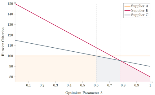
To find the critical values for the Optimism Parameter, the intersections of these 3 functions have to be determined. Equating the functions leads to the following values for λ:


Figure 2 shows a graphical represenation of these functions. It can be seen that there are three sections in the diagram depending on the λ value. From the Minimax approach (λ=0) until the intersection of the function for Supplier A and C supplier A will be chosen, since it shows the lowest value in this region. After that, supplier C becomes more attractive and will thus be picked as a resulting decision. However, after the intersection between the functions for supplier B and C it is superseded by Supplier B, with Supplier B staying the most attractive option until the Maxmimax approach (λ=1). While it was already clear after the Minimax and the Maximax approach, how the project manager would decide in the extreme cases (λ=0 and λ=1), a new insight could be gained by examining the Hurwicz criterion using a sensitivity analysis: Picking Supplier C can also be an option if the Optimism parameter lies between 0.600 and 0.778, which indicates a required above-average risk attitude by the project manager.
The next approach will determine the optimal alternative according to the Minimax Regret principle: Since there are no parameters to alter, the result can directly be calculated. Supplier A will be chosen in this case, since it has the lowest opportunity costs (which means the highst opportunity income), followed by Supplier C and then B. This approach is an extension of the basic Minimax Criterion, since it compares the alternatives with each other for each scenario instead of for only one outcome. Thus, it should be used for decisions where the risk of unexpected increased costs should be kept low.
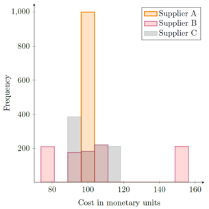
Since the scenario that will occur is uncertain, it can be modelled by generating random numbers. In this case, a random number from 1 to 5 was produced and then attributed to the respective costs for each supplier for the scenario matching the random number. This Simulation was run 1,000 times to ensure a comparably stable result. The results are illustrated in a histogram in figure 3.
Since Supplier A shows no deviation depending on the scenario, all 1,000 results yielded a cost of 100 monetary units. Comparing Supplier B and C makes clear that Supplier B shows a wide spread around the estimated costs, while Supplier C stays closer to the average. The reason that Supplier C shows a comparably high occurence of cases with a cost between 88.75 and 96.25 is that both Scenarios 1 and 2 fall into this range. Another insightful information can be the comparison of the average values for the Monte Carlo Analysis per supplier with the respective Laplace Criteria, which the following table shows:
| Issue examined | Supplier A | Supplier B | Supplier C |
|---|---|---|---|
| Laplace Criterion | 100.00 | 106.00 | 102.00 |
| Monte Carlo Sim. | 100.00 | 106.58 | 102.40 |
| Deviation | 0.00 % | 0.55 % | 0.39 % |
It is noticeable that for 1000 simulated values the deviations are miniscule and calculating the mean value results in the same result as the Laplace approach. Considering the simulated distribution together with this finding, the project manager should pick Supplier A due to lower average costs as well as the narrowest distribution. This procedure provides both an overview about the mean costs of decision alternatives as well as about the respective distributions and can thus be used to get a better understanding how the scenarios affect the respective outcomes.
A point that can be critisized is that only the costs were considered in this example and not features like reliability or service quality. Also, all the outcomes were assumed to have an equal probablity of happening which is rather unrealistic. Especially considering scenario 5 equally probable put a high weight on the 150 monetary units of Supplier B for this scenario. However, for minor supplier selection decisions these approaches provide results with low effort. Concluding this section, the selection of the approach for a problem depends on the risk the project manager wants to take and the information she is trying to extract. In order to get a better understanding of the consequences of a selection, performing different approaches to make a decision is recommended. [3]
Limitations
.
Annotated bibliography
.
References
- ↑ 1.0 1.1 Shaltry, P. E. (2009). Book Review: The Project Manager’s Guide to Making Successful Decisions. Project Management Journal, 40(4), 107–107.
- ↑ Züst, R., & Troxler, P. (2006). No More Muddling Through. Springer Netherlands. https://doi.org/10.1007/978-1-4020-5018-3
- ↑ 3.0 3.1 Kerzner, H. R. (2017). Project management: A systems approach to planning, scheduling, and controlling (12th ed.). John Wiley & Sons.
- ↑ 4.0 4.1 Renou, L., & Schlag, K. H. (2010). Minimax regret and strategic uncertainty. In Journal of Economic Theory (Vol. 145, Issue 1, pp. 264–286). Elsevier BV. https://doi.org/10.1016/j.jet.2009.07.005
- ↑ 5.0 5.1 5.2 5.3 5.4 Chung ES, Kim Y. Development of fuzzy multi-criteria approach to prioritize locations of treated wastewater use considering climate change scenarios. J Environ Manage. 2014 Dec 15;146:505-516. doi: 10.1016/j.jenvman.2014.08.013. Epub 2014 Sep 11. PMID: 25218330.
- ↑ Maclean, F. I. (1987). Rectangular game theory and metabolic response to random changes in environmental states. In Biosystems (Vol. 20, Issue 3, pp. 259–266). Elsevier BV. https://doi.org/10.1016/0303-2647(87)90033-5
- ↑ Geronymakis, P., Troullinos, D., Chalkiadakis, G., & Papageorgiou, M. (2022). Collaborative Decision Making for Lane-Free Autonomous Driving in the Presence of Uncertainty. In Multi-Agent Systems (pp. 171–187). Springer International Publishing. https://doi.org/10.1007/978-3-031-20614-6_10
- ↑ Bennett, N., & Axelos. (2017). Managing successful projects with PRINCE2 (The Stationery Office, Ed.; 6th ed.). TSO.
- ↑ Jiang, Z.-Z., Zhang, R., Fan, Z.-P., & Chen, X. (2014). A fuzzy matching model with Hurwicz criteria for one-shot multi-attribute exchanges in E-brokerage. In Fuzzy Optimization and Decision Making (Vol. 14, Issue 1, pp. 77–96). Springer Science and Business Media LLC. https://doi.org/10.1007/s10700-014-9189-x
Cite error: <ref> tag with name "Fang2021" defined in <references> is not used in prior text.


