Feasibility risk assessments of transport projects using Monte Carlo-simulations

Abstract

A common way of assessing the feasibility of an infrastructure projects (e.g., road or rail) is through a cost benefit analysis (CBA), resulting in an overview of the cost and benefits/ consumer surplus as the Net present value (NPV) or Benefit cost ratio (BCR) of the project. Values which can be compared to other projects/alternatives. The result of a CBA though relies on a single value where all assumptions, estimations and calculations are reduced to a single number. It can thus be difficult to describe the certainty of the result and due to the complexity of infrastructure projects a risk of cost overruns and overestimations of benefits are historically likely to occur . One way to challenge this problem is to perform a Feasibility risk assessment (FRA) moving from a single point result to an interval result.

One FRA technique trying to cope with some of the shortcomings of CBA are a stochastic approach based on Monte Carlo simulations using reference classes. Also called reference scenario forecasting (RSF). The idea of using reference classes is to gather all possible information regarding already implemented infrastructure investment projects, which thus can be used to provide a background for evaluation of future projects and identify probability distributions that can model the uncertainty of the project impacts. .

The result of the FRA using Monte Carlo simulation is a certainty graph and/ or certainty interval providing information about the certainty of achieving e.g., a BCR of at least one. That is potentially valuable information for decision makers describing in how many cases or how large the certainty is of obtaining a project that is feasible.

This article will describe how FRA can be implemented and support decision making within transport projects. Other areas where Monte Carlo simulation can be used is to determine the schedule of a project.

Reasoning behind and optimism bias

Figure 1: Decision support model towards the feasibility risk assesment

In order to get a social, environmental, and economical acceptance of an infrastructure project an assessment of the impacts is necessary. This includes travel time savings, emissions, accidents etc. as well as construction and maintenance cost summarised in a Cost Benefit analysis (CBA). The CBA has the advantage that it through the provided set of criteria sums up all aspects of the decision problem to one single monetary value, net present value and/or benefit cost ratio, and make the variety of projects comparable and consistent.

This though may also be considered a weakness as the methodology might be seen as a “black box” reducing all considerations and assumptions to one single value. Furthermore, the unit pricing principles and modelling of impacts involves uncertainties due to the unknowns of the future . Thus, the CBA only provides a single guesstimate on the feasibility of the project.

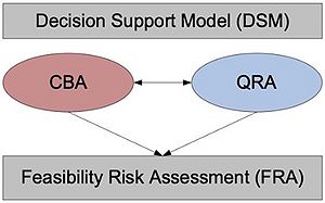
Megaprojects are inherently risky due to long planning horizons and complex interfaces and a systematic tendency to overstate some of the major impacts, such as user benefits and construction cost are demonstrated. This is also known as “optimism bias” where lessons learned are likely to be neglected with a with a common belief that the future will be better than the past and that ‘the same mistake won’t happen twice'. The traditional way of handling the above-described uncertainties is through a risk analysis. Here, the undesirable effects that the subsequent activities may impose are identified and quantified in a risk matrix and mitigation measures are determined. Each single project is thus handled as a unique project identifying what may go wrong within this context. The traditional Risk analysis of course gives some useful insights and provides the decision maker with a method by which he/her can gain information on the totality of any future outcome. By adding a quantitative risk analysis (QRA) it provides the possibility to differentiate the feature of risk information in terms of outcome by probability distributions and provide an indication of the degree of overall risk faced by the project, portfolio, or program. While the CBA is appealing to its adaptability and flexibility it often applies a ‘false sense of security’ where underlying model uncertainties are somehow forgotten. Complementing the CBA with a QRA in a “feasibility risk assessment” (FRA) thus provides additional knowledge on the viability of a project and handle the uncertainties present in the decision making by moving from a single point result in the CBA to an interval result with a corresponding probability. The result can further be used to estimate any contingency reserve.

Application

The structure of the QRA is similar to a deterministic single value rate of return model but instead each input variable (e.g., cost drivers) in the model is represented by a probability distribution function. By a random sampling method several scenarios (also called iterations) can be produced concerning different probability distributions and the outcome of the model thus reflects the probability of achieving a feasible project and at what extent. One technique, presented in the following, highly suitable for a QRA model is reference scenario forecasting using Monte Carlo simulations .

Monte Carlo simulation

Running a RSF as a Monte Carlo simulation is an “analytical technique used to show the combined effect of uncertainties in order to evaluate their potential impact on objectives” .

Monte Carlo simulation is a stochastic simulation where random samples or ‘draws’ (numbers) of input variables are generated from a particular predefined distribution and forms the basis of hundreds or thousands “what-if” scenarios.

Choosing distribution

The main input variable in the FRA to be simulated are the cost (e.g., construction cost) and the user benefits (e.g., travel time savings) derived from the CBA. These are usually two major posts in transport projects and an over/underestimation is a risk that can have a major impact in the feasibility of the project. It is thus crucial to attain applicable data (hence, distributions) when working with Monte Carlo simulations.

Two forms of data that can be applied are expert judgment or historical data. In transport projects expert judgement are usually applied when conducting risk analysis of accidents or maintenance cost while historical data can provide knowledge of construction cost and travel time savings of similar projects.

Identifying the most appropriate probability distribution to simulate (historical or expert) data is done through data fitting. It can however be difficult to determine the exact distribution to apply and thus, different goodness of fit tests is needed.

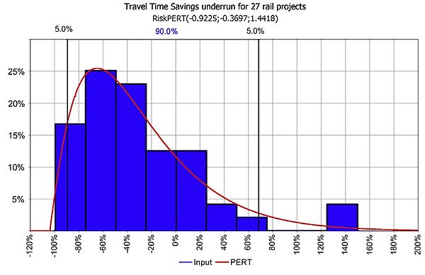
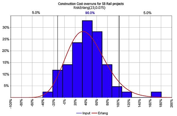
Several research and case studies varying from air, rail to road projects have been made made by Flyvbjerg et al. 2003, to find and validate suitable data and distributions describing different transport impacts as construction cost and travel time savings . . Some of the applied data fits are presented in figure 2 and 3 .

Figure 2: Inaccuracy of travel time savings in rail projects

Figure 2 shows a sample of 27 rail projects and the under/overestimation of travel time savings. The blue bars illustrates the inaccuracy of travel time savings. A clear skewness to the right is shown. In this case it was found by Flyvbjerg et al. that a PERT distribution with a high degree of skewness provided a valid fit, represented by the red curve . The values shown at the top of the figure are the data point fit showing a range of -92 % to 144 % with an average of -37 % of inaccuracy in estimated vs. realised travel time savings. Hence, a clear tendency of overestimation .

Figure 3: Inaccuracy of construction cost estimates in rail projects

In figure 3 the realised construction cost compared to the planned construction cost of 58 rail projects analysed in the case study by Flyvbjerg et al are presented. A positive sign depicts a cost overrun. The tendency is, again, skewed with an average of 45 % cost overruns for rail projects. The red curve represents the derived data fit against an Erlang distribution with a shape parameter k = 23 and scale parameter Ѳ = 0,075. The shape parameter depicts the skewness of the of the distribution. It is suggested that a shape parameter in the range of k = 4-9 matches the general uncertainty distribution determining construction cost while a much higher shape parameter should be applied for rail infrastructure projects to achieve a descent goodness of fit .

From the case study made by Flyvbjerg et al. it is suggested that, In general, a parametric distribution (e.g., normal, gamma and beta) should be used, if the parameter is specified in literature or historical data while a non-parametric distribution (e.g., triangular or uniform) should be used if the parameter relies on judgment of the uncertainty by experts. Using a parametric distribution further care should be taken securing that:

• the chosen distribution applied to the problem is supported by theory.

• it has been proven beneficial to apply the chosen distribution through a general acceptance of the problem.

• the chosen distribution approximately fits the expert’s opinion being modelled and the required level of accuracy is not too high .

Figure 4 summarises the case study distributions found suitable for application on various transport parameters and can be used to assists the choice of the most suitable distribution. The source refers to the source of the uncertainty .

Figure 4: List of suggested probability distributions

While it is preferable to assign distributions as a result of a data fit, this is often not possible since data are sparse. It all comes down the level of knowledge about realised impacts of already implemented projects. It can thus be beneficial for an organisation to establish a project database for future reference class forecasting including information about estimated construction cost, estimated user benefits and other impacts as well as the actual construction cost and the realised benefits/impacts.

Running the Monte Carlo simulation

While software Python or R studio are commonly used to run Monte Carlo simulation and subsequent FRA it requires some knowledge in programming. However, a Monte Carlo simulation can easily be run through build-in functions in Microsoft excel.

The following will describe how random sampling of travel time savings and construction cost as these are the major impacts of infrastructure projects. However, a further break down of e.g., user benefits could be made in order to do random sampling of e.g., time and travel distance savings, while externalities could be broken down into accidents and pollution.

In excel a column for simulation number, Consumer surplus, Construction cost (etc) are defined. The first input needed for the simulations is the socio economical posts derived from the CBA as consumer surplus (travel time savings converted to monetary value) and construction cost. (other posts such as scrap value, maintenance cost, and externalities could be included).

A rail project is e.g., estimated to cost 2.750.000.000 DKK. The consumer surplus is estimated to be 3.130.000.000 DKK

Next the parameters for the chosen distribution is needed. The parameter for this example is derived from the previous mentioned case study made Flyvbjerg et al. 2003

Simulating the consumer surplus (travel time savings) a “Beta-Pert” distribution is chosen which needs parameters for the minimum, most likely, and maximum deviation of estimate.

A is calculated as: 1+Minimum

1+(-0,92) = 0,08

B is calculated as: 1+Most likely

1+(-0,37) = 0,63

C is calculated as: 1+Maximum

1+1,44 = 2,44

alpha=\frac{4(b-a)}{(c-a)}+1 (4(0,63-0,08))/(2,44-0,08)+1=1,94

beta= (4(c-b))/(c-a)+1

	(4(2,44-0,63))/(2,44-0,08)+1=4,06

The consumer surplus can now be simulated running the following excel function:

=Beta.INV(Rand();alpha;beta;a;c)*CBA_consumersurplus

=Beta.INV(Rand();1,94;4,06;0,08;2,44)* 3.130.000.000

Simulating the construction cost an “Erlang” distribution is chosen which needs a shape and a scale parameter.

The shape parameter k = 23

The scale parameter Ѳ = 0,075

The construction cost can now be simulated running the following excel function:

=Gamma.INV(Rand();shape;scale)*CBA_construction_cost

=Gamma.INV(Rand();23;0,075)* 2.750.000.000

In order to achieve a ‘stable’ certainty graph (see below) a good rule of a thumb is to run (at minimum) 2.000 Monte Carlo simulations . Upon the 2.000 simulations of consumer surplus and construction cost a benefit cost ratio (BCR) can be calculated for each simulation (in a new array in excel). The benefit cost ratio is a summation of all project benefits divided by the construction cost .

Certainty graph

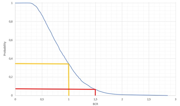
The result of running an FRA using Monte Carlo simulations is, as mentioned, a bunch of ‘What-if’ scenarios testing different combinations of construction cost and user benefits and the resulting benefit cost ratio (BCR). The simulated ‘scenarios’ can be summarised in an cumulative descending graph, or so-called ‘certainty graph’. The advantage of a certainty graph is that it provides the decision maker with a visual reference from which it is fairly easy to interpret the certainty of the project’s feasibility / or the risk of being unfeasible.

The certainty graphs are derived by finding the BCR for a given probability (0,0 to 1,0) in steps of 0,01. This is done by applying Excel’s percentile function to the array of simulated BCRs:

=PERCENTILE(BCR_Array;(1-probablility))

The certainty graph is central means of communication in an FRA . Figure 4 illustrates the probability (y-axis) of achieving a certain benefit cost ratio or higher (x-axis). Hence moving the vertical orange line upwards on the blue graph the lower the risk while the BCR however decreases.

Figure 4: Certainty graph of 2000 Monte Carlo simulations. With red, the probability of realising a BCR of 1,5 (Stated by the CBA). With orange the probability of realising a BCR of 1

As an example, let’s say, that the analysed project yielded a BCR of 1,5 according to the cost benefit analysis (CBA). In order of a project being (economically) feasible a BCR of at least one must be achieved. Hence, according to the CBA only, the project is feasible. However, running an FRA it can be derived by the certainty graph, that the probability of achieving a BCR of 1,5 or more is 8 % (red line in figure xx), while the probability of achieving a BCR of 1 or more is 32 % (orange line). Thus, the risk of the project actually being infeasible is 68 %.

Running the FRA clearly states, that the CBA might not provide all the information needed in order to make a decision of running a certain infrastructure project. The FRA thus provides decision makers with additional information of the risks of the project being infeasible based on e.g., historical data.

Limitations

When performing a feasibility risk assessment it is necessary to distinguish whether it’s a road or railway project. This is usually not an issue, however, some large infrastructure projects might include both. In this case it becomes slightly more difficult to perform the FRA as it is necessary to consider the construction cost and user benefits (and other costs/benefits) independently on the two modes in order to apply the right parameters when running the Monte Carlo simulation. Subsequently the costs and benefits simulated separately for each mode must hereafter be summarised in a “single” benefit and cost value respectively for every simulation run in order to evaluate the overall feasibility of the project. Hence, if its chosen to run e.g., 2000 Monte Carlo simulations for the project it is thus needed to run 2000 simulation for each mode and thereafter combine the outcomes.

As described previously the parameters/distribution chosen relies on the reference classes. Hence, there must be similarities between the project at hand and the references. The current presented research does not provide a general guideline on how to define the level of similarities when choosing reference scenarios and it is thus up to the project/ risk manager to decide which scenarios to include. While it could be discussed whether e.g., a railway tunnel between two islands should be included as a reference scenario evaluating a new railway on land, an assessments of what reference scenarios to include also implies that a new data fit and definition of distribution parameters is needed which requires additional work.

One of the greater disadvantage of the FRA is the requirement of realised benefits (and cost) of an already finished project. This requires a post analysis which a major task in itself. At the same time post analysis of transport projects are usually made on highly successful projects and projects of complete failure while those in between are somewhat forgotten.

The FRA is a useful technique to supplement a cost benefit analysis providing decision makers with a better understanding of the sensitivity of the CBA and consequence of potential cost overrun and/or wrong estimated user benefits.

While a project might have a high risk of not being feasible in a FRA it must be noted that assessments only relies on the results from a CBA. Thus, other criteria’s as e.g., urban development, Environmental impact, etc. should also be considered through a more extensive analysis combining a CBA with a multi criteria analysis before concluding on the overall feasibility of a project.

Conclusion

A cost benefit analysis is a highly useful tool when making investments appraisals of transport projects. However, the CBA only returns a single value while significant uncertainties related to parameters/impacts included in the CBA aren’t visible in the result. To mitigate this a feasibility risk assessment (FRA) can be conducted. Running Monte Carlo simulations can generate several “what if” scenarios based on e.g., historical data and provide useful knowledge about the probabilities of actually achieving the project outcome stated by the CBA. Running Monte Carlo simulations though also implies one difficulty of the FRA with the need to consider which probability distributions to be used simulating different impacts.

Other application areas

Monte Carlo simulation can be used to simulate many different areas within risk handling and project managing. Another application area is project scheduling in order to derive the risk of a project or subtask being delayed. The input simulating a project schedule would e.g., be the most pessimistic, most optimistic, and most likely amount of time needed to finish a specific task. Running multiple iterations of every single task within a project, and adding tasks dependencies, it would then be possible to generate several outcomes of the overall project schedule. The simulated project schedule can hereafter e.g., be plotted on a histogram showing the distribution of possible project durations. The project managers is thus able to e.g., identify the time needed finishing the project within a specific level of confidence or in order to specify/ add a contingency reserve.

References

- ↑ 1.0 1.1 “http://wiki.doing-projects.org/index.php/Risk_Assessment:_framework_for_combining_CBA_and_MCDA”
- ↑ “Flyvbjerg, B., 2014. What You Should Know About Megaprojects and Why: An Overview. Oxford University”
- ↑ 3.0 3.1 3.2 3.3 “Leleur, S., Salling, B., 2012. Modelling of Transport Project Uncertainties: Feasibility Risk Assessment and Scenario Analysis. Department of Transport, Technical University of Denmark”
- ↑ 4.00 4.01 4.02 4.03 4.04 4.05 4.06 4.07 4.08 4.09 4.10 4.11 4.12 “Barfod, M. & Leleuer, S., 2021, Decision Support and Strategic Assessment, DTU management”
- ↑ “HM Treasury, 2022, The Green Book: CENTRAL GOVERNMENT GUIDANCE ON APPRAISAL AND EVALUATION”
- ↑ “Salling, B., 2008, Assessment of Transport Projects: Risk Analysis and Decision Support, DTU Management”
- ↑ “Project Management Institute, Inc., 2019, Standard for Risk Management in Portfolios, Programs, and Projects”
- ↑ “Project Management Institute, Inc, 2021. A guide to the Project Management Body of Knowledge (PMBOK guide), 7th Edition”
- ↑ 9.0 9.1 Leleur, S. Salling, B., Pilkauskiene, I. & Nicolaisen, M., 2015, Combining Reference Class Forecasting with Overconfidence: Theory for Better Risk Assessment of Transport Infrastructure, Technical University of Denmark & Aalborg University
- ↑ 10.0 10.1 10.2 10.3 10.4 10.5 10.6 Flyvbjerg, B., Bruzelius, N. & Rothengatter, W., 2003, Megaprojects and Risk – An anatomy of Ambition. Cambridge University Press, United Kingdom.
- ↑ 11.0 11.1 11.2 11.3 11.4 11.5 Salling, B. & Banister, D., 2009, Assessment of large transport infrastructure projects: The CBA-DK model. Technical University of Denmark, Oxford University