Test15

Decision making is one of the most important tasks in the management process and it is often a very difficult one. When having knowledge regarding the states of nature, subjective probability estimates for the occurrence of each state can be assigned. In such cases, the problem is classified as decision making under risk . In the decision making process, all relevant information is evaluated through decision analysis (DA). The decision analysis process consist of the use of a decison tool and a decision theory. The decision tree is the most commonly applied decision tool in the decision analysis . The decision theory of interest in the decision analysis, regarding the decision making under risk, is the expected value of criterion also reffered to as the Bayesian principle. This is the only one of the four decision methods that incorporates the probabilities of the states of nature .

---

Methologdy

Risk analysis and risk management is an important tool in the construction management process. Risk implies a degree of uncertainty and an inability to fully control the outcomes or consequences of such an action. The objective of a decision analysis is to discover the most advantageous alternative under the circumstances .

Decision analysis is a management technique for analyzing management decisions under conditions of uncertainty . The decision problems can be represented using different statistical tools applied to the mathematical models of real-world problems. An important and relevant decision tool to represent a decision problem is a decision trees. A decision tree is a graphical representation of the alternatives and possible solutions, also challenges and uncertainties. In decision analysis, formulating the decision problem in terms of a decison tree is a favorable visual and analytical support tool, where the expected values of competing alternatives are calculated.

Theory and principles

The following provides the theory and principles behind the decision making under risk, using bayesian decision analysis. An overview of the principles and construction regarding the decision tree is provided as well as a the decision theory regarding the decision tree analysis.

Decision tree

A decision tree (DT) is a chronological representation of the decision process. It is particularly useful where there are a series of decisions to be made and/or several outcomes arising at each stage of the decision-making process, it is therefore useful in analyzing multi-stage decision processes. The number of alternative actions can be extremely large and a framework for the systematic analysis of the corresponding consequences is therefore expedient. Decision trees is an effective decision tool in the decision-making, because it:

Figure 1: Decision tree diagram (click to zoom)

• Clearly lay out the problem so that all options can be challenged
• allow to fully analyse the possible consequences of a decision
• provides a framework in which to quantify the values of outcomes and the probabilities of achieving them
• helps make the best decisions on the basis of existing information and best guesses.

A decision tree is a schematic, tree-shaped diagram representation of a problem and all possible courses of action in a particular situation and all possible outcomes for each possible course of action. The diagram is constructed of branches and each branch of the decision tree represents a possible decision, occurrence or reaction. The tree is structured to show how and why one choice may lead to the next, with the use of the branches indicating each option is mutually exclusive.

A decision tree consists of three type of nodes, there is no universal set of symbols used when drawing a decision tree but the most common ones is:

• Decision (choice) Node – square
• Chance (event) Node - circles
• Terminal (consequence) Node – triangles

Construction of decision tree

For the purpose of illustrating the construction of a decision tree, based on the illustrated diagram on figure 1, the following consideres a simple decision problem. An old bridge has been subject to deterioration, control data reveal that the bridge structure may be damaged. However, this cannot be indicated with certainty. If the bridge is damaged, it is unfit for service and a new one needs to be constructed. Your company is hired to find the best solution of two alternatives:

1. Alternative a₁: Do nothing
2. Alternative a₂: Repair the bridge

The decision analysis is therefore to evaluate weither is most beneficial to do nothing or repair the bridge, so which alternative is associated with the lowest risk, in this case the lowest risk is the alternative with the lowest expected cost.

Figure 1: Risklevel (click to zoom)

Figure 2 illustrates the construteced decision tree for the giving example. The illustration is constructed by the author using a 'DPL9' which is a decision tree making program (reference til hjemmesiden).

1. The first node drawn is the decision node, a branch emanating from a decision node corresponds to a decision alternative, which in this case are either to repair the bridge or do nothing. It includes a cost or benefit value, which in this example is refered to as cost 1 and cost 2. The decision node is illustrated by a yellow square.
2. The next node is a chance node, since both alternatives does not lead to a new the decision. A branch emanating from a state of nature (chance) node corresponds to a particular state of nature, and includes the probability of this state of nature. For both alternatives the branches has the same outcome, either the bridge is safe and fit for service or the bridge is damaged. The probability associtaed with the bridge being safe or damaged, are denoted P(S1) and P(S2), respectively. The chance node i illustrated by a green circle.
3. The final node is the terminal node, this represent the cost consequens related to the choice of decision branch. The value for the terminal nodes, are the sum of the cost for each branch. This values is also called the net path value (NPV).

Decision theory

Decision theory is an analytical and systematic way to tackle problems. Decision theory is the part of probability theory that is concerned with calculating the consequences of uncertain decisions. This can be applied to state the objectivity of a choice and to optimise decisions .

The decision method used is the expexted value of criterion, it incorporates the probabilities of the states of nature. The expected value criterion, also refered to as expected monetary value (EMV) analysis is the foundational concept on which decision tree analysis is based. EMV is a tool and technique for the “Perform Quantitative Risk Analysis” process (or simply, quantitative analysis), where a numerically analyze is performed regarding the effect of identified risks on overall project objectives. The EMV of risk is:

Expected Monetary Value= Probability of the Risk x Impact of the Risk.

EMV calculates the average outcome when the future includes uncertain scenarios, it is the sum of the different scenarios related to a chance note. The final decisions is therefore based on expected values of the corresponding consequences.

Depending on the state of information regarding the probability at the time of the decision analysis, three different analysis types are distinguished, namely prior analysis, posterior analysis and pre-posterior analysis. Each of these are important in practical applications of decision analysis and are therefore discussed briefly in the following, with the utility is represented in a simplified manner through the costs.

Prior analysis

The prior analysis, is a decision analysis performed with known information, it quantify the beliefs before any evidince is taking into account. At this stage, the probabilistic description $\scriptstyle P[\theta]$ of the state of nature $\scriptstyle \theta$ is usually called a prior description and called $\scriptstyle P'[\theta]$ . When the probabilities of the various state of nature corresponding to different consequences have been estimated, and the consequences for the fianl outcome determined, the analysis consists of the calculation of the expected utilities corresponding to the different action alternatives.

The optimal decision is identified as the expected cost, $\scriptstyle E'[C]$, also called the expected value of perfect information when the decision is based on the prior information,

Posterior analysis

The posterior analysis is the conditional probablilty that is assigned when additional information becomes availble. The conditional probabilities form the basis of updating of probability estimates based on new information, knowledge or evidence, which makes conditional probabilities of interest in risk and reliability analysis.

The conditional probability is the probability of an event, given that another event has already accord. The posterior probability of an event $\scriptstyle \theta_i$ , given that another event, $\scriptstyle A$ , has occured is therefore expresed as:

${P''[\theta_i | A] = \frac {P[A|\theta_i] P' [\theta_i]} {P[A]}}$

The conditional term $\scriptstyle{P[A|\theta_i]},$ can be referred to as the likelihood, the probability of observing a certain state given the true state. The term $\scriptstyle{P'[\theta_i]},$ is the prior probability of the event $\scriptstyle \theta_i$, prior to the knowledge about the event $\scriptstyle A$ ). $\scriptstyle{P[A]},$ is the probability of the event $\scriptstyle A$ , i.e. $\scriptstyle{P[A]},$, can be written as

${P[A]=\sum_{i=1}^n P[A|\theta_i] P' [\theta_i]}$

Having determined the updated probabilities the posterior expected value $\scriptstyle E''[C|A]$ is found in order to determine the optimal solution.

Pre-posterior Analysis

The objective of preposterioe analysis is to determine the whether the value of the prediction is greater or less than the cost of the information. Posterior refers to the revision of the probabilities and the pre indicates that this calculation is preformed before paying the fee. The goal is therefore to choose the experiment or experimental design which minimixe the overall cost . The preposterier analysis is based on the expected value,

${E[C]=\sum_{i=1}^n P'[A_i] E'' [C |A_i]}$

The posterior expected cost $\scriptstyle {E'' [C |A_i]}$ therefore needs to be determind in the proces of prefroming the pre-posterior analysis.

Baysian decision analysis

The theory and principles of decision making under risk, has been represented. An example with is now presented with the applied theory.

Example 1 - Prior analysis

The prioir analysis is related to the condition of known information. Using the same example as given previous under the construcion of the decision tree, following information is now provided:

It is estimated that there is a 10% probability that the bridge structure is safe. If the bridge is repaired then the probabaility of the bridge stucture having damaged is 20%. Table 2 provides the probabilities used in the construcion of the decision tree in figure 3.

	a1- Do nothing	a2- Repair bridge
$\scriptstyle P[\theta_1]$ - Safe	0.1	0.8
$\scriptstyle P[\theta_2]$ - Damaged	0.9	0.2

Table 2: Probabilities related to the two alternatives

Figure 3: Decision tree example 1 - prior analysis (click to zoom)

If the bridge structure is damaged, then a new bridge is reqiured which is asssociated with a cost of $100 mio. If the structure is safe then the cost is $0. If it chosen to repear the bridge, cost of the the reperation costs $20 mio. Looking at figure 2, the value related to cost1 is $0mio. and cost2 is $20mio. Providing the informations regarding the costs and the probabilities, the decision tree related to this case can be seen in figure 3. The program calculates the net pressure value, the value at the end nodes, when the decision analysis is preformed. Therefore the branches are provided with their individual, related values. For simpicity the net pressure values are shown in table 3.

	NPV
NPV 1	$0mio.
NPV 2	$100mio.
NPV 3	$20mio.
NPV 4	$120mio.

Table 3: Net path values (NPV) for example 1.

In this example the utility is represented in a simplified manner through the costs whereby the optimal decisions is identified as the decisions minimizing expected costs, which then is equivalent to maximizing expected utility.

The decision analysis is preformed using EVM, the calculations are done from left to right, starting with the chance nodes having branches ending in the final nodes.

1. chance node - associated with alternative a ₁ '

The decision tree analysis is now preformed,

$\scriptstyle EVM_1=P[\theta_1] * NPV_1 + P[\theta_2] * NPV_2=0.1 * $0mio. + 0.9 * $100mio.= $90mio.$

2. chance node - associated with alternative a ₂ '

$\scriptstyle EVM_2=P[\theta_1] * NPV_3 + P[\theta_2] *NPV_4= 0.8 * $20mio. + 0.2 * $120mio. = $40mio.$

The optimal decisions based on the prior information, is identified as the decisions minimizing expected costs. Therefore

$\scriptstyle E'[C]=min{EVM _{a ₁};EVM _{a ₂}}=$40mio.$

Alternative a ₂ , repair the bridge....

Figure 4 show results of the decision analysis preformed in DPL9. In figure 4 the net path values are given at the terminal nodes, as well as the expected values at the chance nodes. The branch representing alternative a ₂ , is bold, confirming decision way.

Example 2 - Prosterior analysis

When additional information becomes available, the probability structure in the decision problem may be updated. Having updated the probability structure the decision analysis is unchanged in comparison to the situation with given prior information. The same condition and information provided in example 1 is used. Now acquired more information through a study about the chances of a bridge repairment. The study costs $5mio. Table 4 contains the estimation of the success rate (structure safe) of the bridge repairations in the study. Bridge repairment results 𝑆 (structure safe) 𝑆̅(structure damaged) Indication 𝐼 90% 10%

Table 4: Study indication of bridge repairment success.

Given the result of the study, the updated probability structure or the posterior probability,now called P'(S) is evaluated by use of the Bayes' rule. P ��[θi] = P[I| θi]P[θi ]�j P[zk| θj ]P�[θj ]

P[I]=

The decision tree is now updated and is presented in figure 3.

The cost for the repairment of the bridge is now changed to $25mio., since is is both the cost of the repairent and the study.

This now give:

Compared to the prioir analysis, the new The prerior analysis is related to the condition of known information. Using the same example as given previous under the construcion of the decision tree, following information is now provided: If the bridge structure is damaged, then a new bridge is reqiured which is asssociated with a cost of $100 mio. If the structure is safe then the cost is $0. It is estimated that there is a 10% probability that the bridge structure is safe. If the bridge is repaired then the probabaility of the bridge stucture having damaged is 20%. Reparing the bridge costs $20 mio. Table 1 provides the probabilities used in the construcion of the decision tree in figure 2.

	a1- Do nothing	a2- Repair bridge
P(S1) - Safe	0.1	0.8
P(S2) - Damaged	0.9	0.2

Table 1: Probabilities related to the two alternatives

The cost for reparing the bridge is $20mio, which means that cost1=$0mio. and cost2=$20mio.. Providing the given values in figure 1, the decison tree is now represented in figure 2.

• 

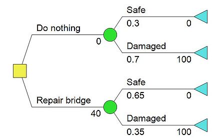  Figure 2 - Decision tree

The pogram used is having the cost related to each branch, which means that value for the terminal nodes, are the sum of the cost for each branch. This values is also called the Net Path value or NPV. The values are shown in figure 3 and futhermore presented in table 2 below.

NPV	Cost-
NPV 1	$0mio.
NPV 2	$100mio.
NPV 3	$20mio.
NPV 4	$120mio.

Table 1: Net path values (NPV) for example 1.

The decision tree analysis is now preformed, starting with first chance node, associated with alternative a ₁ . EVM=P(s1)*0 + P(s2)*$100mio=$90mio Chance node 2 EVM=P(s1)*$120mio + P(s2)*$120mio=$40mio

The most benifical solution, is the one associated with the lowest cost, so:

E[C]=min{EVM _{a 1 ;EVM a 2 }.}

Example 3 - Pre-Postrior analysis

Often the decision maker has the possibility to ‘buy’ additional information through an experiment before actually making his/her choice of action. If the cost of this information is small in comparison to the potential value of the information, the decision maker should perform the experiment. If several different types of experiments are possible, the decision maker must choose the experiment yielding the overall largest expected value of utility. The conditional probability is used in the pre-posterioe analysis, for the simplicity a new example is taken is taken

Karabadji, Nour El Islem et al. “An Evolutionary Scheme for Decision Tree Construction.” Knowledge-based Systems 119 (2017): 166–177. Web. (basis for decision tree)

R.C. Barros, A. de Carvalho, A.A. Freitas, Automatic Design of Decision-Tree

Induction Algorithms, SpringerBriefs in Computer Science, Springer International Publishing, New York City. URL https://books.google.co.kr/books? id¼PFqEBgAAQBAJ, 2015.

Delmar, M.V., and J.D. Sorensen. “Probabilistic Analysis in Management Decision Making.” Proceedings of the International Offshore Mechanics and Arctic Engineering Symposium 2 (1992): 273–282. Print.

Donegan, H. A. “Decision Analysis.” Sfpe Handbook of Fire Protection Engineering, Fifth Edition (2016): 3048–3072. Web.

Khalili Damghani, K., M. T. Taghavifard, and R. Tavakkoli Moghaddam. “Decision Making Under Uncertain and Risky Situations.” (2014): n. pag. Web.

Annotated:

Goodwin, Paul; Wright, George. (2004). Decision Analysis for Management Judgment. Wiley