Financial Portfolio Optimization Methods
Developed by Andreas Kampianakis
In today's globalized market, financial risk and treatment of it that has gained great importance, especially after the Financial crisis of 2008, where factors which may affect the fragile global economy proved to be thousands and often unconnected to each other. Nations fail to pay their debts and giants of the finance industry bailed out [1]. These financial institutions have developed various quantitative methods which can give a prediction of this risk level in financial portfolios. A financial portfolio is considered the summary of investments owned by an investor ( company or individual )[2]. The first step for the quantitative measurement of risk in portfolios was made by Harry Markowitz in 1952 [3], with the development of the mean-variance model as risk measurement, which shows interest until today and it is used by investors. Thereafter, various other methods were developed, focusing on alternative risk measures that could lead to linearization of the portfolio optimization problem [4] . The main principles of risk handing and best profit can be applied in project management.
Contents |
Financial Portfolio Optimization Methods in PPM
In order for a business to minimize the danger of exposure to a failed project, financial portfolio methods can be applied. Consider "assets" to be financial, physical, or information that combined with other assets in a project will increase value. The "group" of assets is designed to achieve the growth of value at acceptable levels of risk over the longer term. The "investor" is a business manager whose job it is to put assets to function efficiently as a portfolio [5]. Each of Markowitz’ principles in Modern Portfolio Theory (MPT) were translated into a criterion for project prioritization that aids in the success of project portfolio management (PPM). In modern project portfolio management, other than risk and return, there are elements such as benefits maximization, balance, strategic alignment and resource leveling. Application of methods of financial portfolio optimization can help a project manager to evaluate projects taking in consideration the interaction and influence of other projects.[6]

Models of Optimization
Background
The term efficient portfolios was developed in the 1950's by Harry Markowitz [3], [8]. An efficient portfolio is one that at given level of risk provides the greatest return and at given performance holds the less amount of risk. According to this definition, an investor will choose from a set of possible portfolios, the portfolio which:
- offers the maximum expected return for different levels of risk
- offers the lowest risk for different levels of expected return.
Those portfolios that meet the before-mentioned requirements are considered as effective ones. Figure 2 shows an example where all the possible portfolios which are formed based on the expected return and risk relations. The set of efficient portfolios has the form of a parabola in between the axes of the expected return (vertical axis) and the level of risk (horizontal axis). Points A, B, C, D, E, F, show some of the possible portfolios. Of all the available portfolios, the most efficient ones are those found in upper left part of the curve of efficient portfolios between A and F. All other portfolios are regarded as ineffective. For example, the A portfolio excels E because it offers the same performance with less risk. Similarly the C portfolio excels D because it offers more return at the same risk level.

Assumptions
A series of assumptions regarding the market and investors were made in order to quantify risk [9] [10]
- Investors are "reasonable" and behave in such a way to maximize their benefits according to the available capital.
- Investors have free access to a fair and accurate information concerning risk and expected returns.
- Markets are efficient and absorb information quickly and perfect.
- Investors avoid risk through the effort to maximize the profit and minimize the danger of investments.
- Investors base their decisions in accordance with the expected performance and a mathematically defined risk measure.
- Investors prefer higher returns than lower ones at a given risk levels.
Mean Variance Model
This model of optimization financial portfolios was the beginning of Modern Portfolio Theory and was the cornerstone for the study of risk in securities. It is still used because of its simplicity and its greater degree of physical understanding of the mathematical aspects, however its non-linear nature raises the complexity of solution in order to find the best portfolio [11] compared to models that are linear and will be further discussed below. In the case of this model it is assumed that there are  assets. Each bond
  has expected return
  , the variation of performance is denoted as
  , and
, and  is the co-variance of returns in relation to another security
  . If
. If  is the desired performance of the portfolio then:
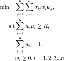
The term  represents the percentage of the capital that will be invested in each bond. This is a quadratic programming problem, and hence the solvability puzzled the financial industry for many years. Today, however, the available computational tools enable the solution of this quadratic program even for large-scale data [11].
Mean Semi-Variance Model
An alternative to the problem of portfolio optimization using mean variance is to use the term of the average semi-variance, a proposal made again by Markowitz [8], [12]. Because an investor is more concerned about minimizing under-performance instead of over-performance, the semi-variance was considered as a more appropriate measure of the risk variance .The difference is that semi-variance measures only downward deflection, not both negative and positive deflections as described in Mean Variance model . This model seeks to identify optimal portfolios considering the expected outcomes of each security and its the semi-variance.[13]. The efficient portfolios of the solution of this problem have little semi-variance for a given expected return, and maximum expected return for a given semi-variance. The set of all efficient portfolios form the efficient frontier in returns / semi-variance graph. The linear minimization problem [11] formulized by the above is:
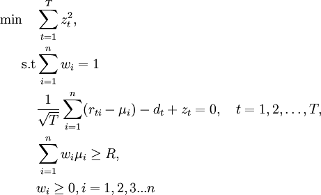
The term  is the rate of return of asset on day
  , and
, and  number of time intervals. Objective function aims to minimize the square of the downside semi-variance
  This formulation led to the first form of utilization of risk of deterioration as a risk measure, which although it is computationally difficult in cases where further restrictions are added [14], it is a quite popular method [15].
CVaR Model
The Conditional Value at Risk, (CVAR) is an extension of the term value at risk (VaR) , in order to create a better estimation of losses in extreme adverse conditions and to address certain theoretical problems of the value at risk [16] . For continuous distributions, CVAR is defined as the expected loss in those cases where the loss of an investment position exceed the corresponding VaR. However, for general loss distributions, including discrete distributions, the CVAR is defined as the weighted average of the VaR and losses that strictly exceed VaR [16]. For general distributions, the CVAR, has more attractive properties from VaR. CVaR is subadditive and convex [16]. In addition, the CVAR has all the essential qualities of a reasonable risk measure, which does not happen in the occasion of VaR, according to Artzner [17], [18]. Although CVaR is not fully accepted in the financial industry, it is gaining ground in the insurance sector [19]. Mathematical formulation of CVaR is [20]:
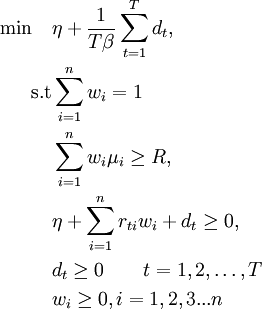
Term  is the investors confidence level as defined in VaR. The term
  is a real variable taking the value of -quantile of the decision variables vector at the optimum[21]. Optimization of CVaR minimizes VaR, since
  .Furthermore another advantage of CVaR against simple VaR is that it can be optimized by linear programming methods and thus creating optimal portfolio can become a process of solving a linear problem which is relatively simple to understand and easy to use as well as its implementation is undemanding [22].
Mean Absolute Deviation Model
The difficulties of solving the model of Markowitz and variants [23] led Konno and Yamazaki in 1988 to present a model consisting exclusively of linear constraints [24], which utilizes as a measure of risk the mean absolute deviation (MAD) . Mean absolute deviation is defined as the average of the absolute deviation from the mean of the data. So the following formula was proposed as risk measure:
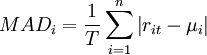
Extending this risk measure to financial portfolios it is observable that because of the absolute nature of risk measurement, the generated problem can not be linear. But it can easily be transformed to one by adding a further variable. So the problem presented for solution is the following:
![\begin{align}
\min \quad & \sum\limits_{t=1}^T y_{t} , \\
\text{s.t} & \sum\limits_{i=1}^n w_{i}[r_{ti}-\mu_{i}]+y_{t} \geq 0 \\
& \sum\limits_{i=1}^n w_{i}[r_{it}-\mu_{i}]-y_{t} \geq 0 \\
& \sum\limits_{i=1}^n w_{i} \mu_{i} \geq R ,\\
& \sum\limits_{i=1}^n w_{i} = 1 \\
& y_{t} \geq 0 \quad t=1,2,3....T \\
& w_{i} \geq 0 , i= 1,2,3...n
\end{align}](/images/math/e/6/3/e6393797f1a09cf420bcd25d483da515.png)
The above modeling helps in examination of a larger number of securities due to the ease in solving a problem of linear constraints as well as the addition of constraints that make it realistic becomes more computationally viable [20].
Additional Constraints
In real situations where investors desire portfolios that meet different realistic features like minimum lots of transactions and transaction costs, solvability of linear models is a critical aspect. Even if the solution of quadratic models like Mean Variance and Semi-Variance has been treated for restrictions in the total number of shares and minimum transactions lots [25] [20], the computational challenge to solve the big and realistic portfolio problems justifies the long tradition in literature of mixed integer programming for portfolio selection with pragmatic characteristics [26] [27] [28]. The models extend the basic portfolio optimization models and result to increased complexity and difficulty of solution. However, the analyzes carried out are closer to reality and the parameters can be adjusted depending on the stock market and investor requirements. Such restrictions can be:
- Restriction in total number of shares. The investor chooses the maximum number of shares they want to invest.
- Limitation of minimum trading lots. The investor virtually round the percentages invested, due to limitations of the financial market.
Transaction roundlots
In any stock market transactions take place in predetermined units (pieces) of each security. Such restrictions are common transactions requirements which means that investing in a security should be expressed as a multiple of a predetermined unit of transaction . The monetary value of each transaction unit is expressed as a percentage of the value of a portfolio [29] so that the composition of the portfolio ( percentage of participation of securities) shall be defined based on these percentages. Moreover limitation of budget becomes "flexible" by the introduction of deviation variables. These variables are denoted as  and
and  , which are minimized in order to limit the budget impbalances as little as possible at the optimal solution [29] [11] . To achieve this, the deviation variables should have very small values [11]. In all models, without exception, the participation grade changes form and it is expressed as
  where
where  symbolizes the transaction module for the security (as a percentage of available capital) and
  is the number of units purchased of the security . In order to implement this particular constraint, each portfolio optimization problem will be converted and the new formulation after the addition of variables mentioned above would be:
where as  determined the objective function of an above-mentioned portfolio optimization model and
  is the set of feasible solutions.
Cardinality constraints
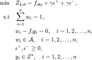
One of the basic assumptions of portfolio theory is that investors can hold well diversified portfolios. However, there are signs that investors typically hold only a small number of securities. Market imperfections such as fixed transaction costs, provide one possible explanation for the selection of undiversified portfolios[30]. Moreover, the need to avoid the costs of monitoring and re-weighting a portfolio leads investors to the common practice of limiting the number of investments (population portfolio securities) that can be selected in a portfolio. The restriction on the number of securities in a portfolio can be expressed either as a strict equality or inequality requiring that the number of selected titles can not be greater than a predetermined number. The addition of the above restriction in each of the models can be done by adding a variable  subject to the following limitations:
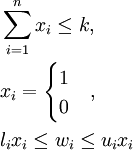
The variable is shown as a binary variable that indicates whether or not the stock participates in the portfolio .  indicates the maximum number of desired stocks and
  and
and  symbolize the lower and upper boundaries respectively, of each participation percentage of a security. It should be mentioned that these constraints are a continuation of the restriction of minimum participation, as developed by Beale and Forrest [31].
Implementations
These basic models of financial portfolio optimization, that basically derive from the Modern Portofolio Theory, seem to have the eligibility to be implemented in more than one applications. The ability to choose the most appropriate set of projects and allocate the amount of in the most efficient way is a desired practical aspect of this mathematical theory. The utilization of MPT in water resource portfolios enabled the researchers to reduce drought problems [32] . Moreover, the same principles were implemented on intervening against the high nutrient loads at the river catchments and had as a main result better budget allocation on environmental investment decision processes [33]. It should also be mentioned the contribution of these model in information retrieval [34] and energy marker [35]. Applications of financial portfolio optimization methods were also implemented in IT industry. The capability of rationalizing risks and maximize profits, is embedded in IBM's tool "Rational Portfolio Manager, as well as in Palisde Corporation's project management tool @RISK. Both of these tools, make use of Monte Carlo Simulation to generate scenarios as input data for the mathematical models mentioned. Modern portfolio theory extensions were also used by Schlumberger , to make optimal portfolio choices of exploration projects (oil wells) having as key aspects the production, investments, cash flows, and geological chance of success[36].
Disadvantages
In literature, it is reported that many of these assumptions do not seem realistic. Assumption of "reasonable investors" often seem to fall short as they generally prefer portfolios different from those resulting from analyzes [37] [38]. Moreover, the grade of complexity becomes greater as the problem grows and its solution becomes extremely difficult or even impossible. Finally, the assumptions mentioned do not take into account the uniqueness of each investor and consider everyone as a unified body, ignoring the behavior that each of them may present. So the difference of institutional and non-institutional investors can lead to values much higher than actual, due to herd behavior in the second category of investors, leading to systematic overvaluation of stock prices [39]. This kind of disadvantages seem to gave birth to various approaches in the problem of portfolio optimization. Fuzzy handling of the problem , seem to solve various of the issues made due to the assumptions such as the nonuniform character of the information among the investors[40] [41] . Moreover multi-criteria analysis haw been implemented in order cope with the investor’s personal attitude towards risk and specific objectives he/she may have [42] [43]. Especially in the field of "non-financial" assets there has been a lot of concern in utilization of such models in order to optimize the project portfolio. First of all, the inability of non divisible allocation , makes the portfolio of projects far more inflexible. This inflexibility makes MPT almost useless. Projects either start or do not, but once they are started there should be an end too. A portfolio optimization method must consider this nature of projects in order to function properly. Also, assets of financial portfolios are liquid; assessment and re-assesement can be done at any point. However opportunity of starting a new project may be limited. Most of the projects that have already started cannot be ceased or sold without the loss of the sunk costs. More specifically, a semi-complete project seems to have no salvation "return", so all the cost of abandonment falls on the shoulders of the investor.[44] [45]. Finally, MPT mostly makes use of a mathematical defined risk measure, but portfolios consisting for example from major building projects do not have a firm one.
See also
- Efficient-Market Hypothesis
- Post Modern Portfolio Theory
- Intertempolar Portfolio Choice
- Decision Theory
- Investment Strategy
- Arbitrage Pricing Theory
Annotated Bibliography
Elton, E. J., Gruber, M. J., Brown, S. J., & Goetzmann, W. N. (2009). Modern portfolio theory and investment analysis. John Wiley & Sons. A book that examines the characteristics and analysis of individual securities as well as the theory and practice of optimally combining securities into portfolios. It stresses the economic intuition behind the subject matter while presenting advanced concepts of investment analysis and portfolio management. Readers will also discover the strengths and weaknesses of modern portfolio theory as well as the latest breakthroughs.
Schwalbe, K. (2013). Information technology project management. Cengage Learning. This book demonstrates the principles distinctive to managing information technology (IT) projects that extend beyond standard project management requirements. The book weaves today's theory with successful practices for an understandable, integrated presentation that focuses on the concepts, tools, and techniques that are most effective today.
References
- ↑ McNeil, A. J., Frey, R., & Embrechts, P. (2015). Quantitative Risk Management: Concepts, Techniques and Tools: Concepts, Techniques and Tools. Princeton university press.
- ↑ [1] Investopedia, Portfolio definition and explanation, Retrieved September 2015
- ↑ 3.0 3.1 Markowitz, H. (1952). Portfolio selection. The journal of finance, 7(1), 77-91.
- ↑ Sharpe, W. F. (1971). A linear programming approximation for the general portfolio analysis problem. Journal of Financial and Quantitative Analysis, 6(05), 1263-1275.
- ↑ Nikonov, O.V, (2007). Efficient Project Portfolio as a tool for Enterprise Risk Management. ERM Symposia
- ↑ Thorp, J. (2003). The information paradox: realizing the business benefits of information technology. McGraw-Hill Ryerson.
- ↑ Bonham, S. S. (2005). IT project portfolio management. Artech House.
- ↑ 8.0 8.1 Markowitz, H. M. (1968). Portfolio selection: efficient diversification of investments (Vol. 16) Yale university press
- ↑ Xidonas, P., Mavrotas, G., Krintas, T., Psarras, J., & Zopounidis, C. (2012). Multicriteria portfolio management (pp. 5-21). Springer New York.
- ↑ Reilly, F., & Brown, K. (2011). Investment analysis and portfolio management. Cengage Learning.
- ↑ 11.0 11.1 11.2 11.3 11.4 Mansini, R., Ogryczak, W., & Speranza, M. G. (2014). Twenty years of linear programming based portfolio optimization. European Journal of Operational Research, 234(2), 518-535.
- ↑ [2]H. Markowitz. The optimization of quadratic functions subject to linear constraints. February 1955
- ↑ Markowitz, H., Todd, P., Xu, G., & Yamane, Y. (1993). Computation of mean-semivariance efficient sets by the critical line algorithm. Annals of Operations Research, 45(1), 307-317
- ↑ Gilli, M., & Këllezi, E. (2002). A global optimization heuristic for portfolio choice with VaR and expected shortfall. In Computational methods in decision-making, economics and finance (pp. 167-183). Springer US
- ↑ Mansini, R., Ogryczak, W., & Speranza, M. G. (2003). LP solvable models for portfolio optimization: A classification and computational comparison. IMA Journal of Management Mathematics, 14(3), 187-220.
- ↑ 16.0 16.1 16.2 Rockafellar, R. T., & Uryasev, S. (2000). Optimization of conditional value-at-risk. Journal of risk, 2, 21-42.
- ↑ Artzner, P. (1997). Applebaum, D.(2004). Lévy Processes and Stochastic Calculus (Cambridge University Press). Artzner, P., Delbaen, F., Eber, J.-M. and Heath, D.(1997). Thinking coherently, Risk 10, pp. 68–71. Risk, 10, 68-71.
- ↑ Artzner, P., Delbaen, F., Eber, J. M., & Heath, D. (2002). Coherent Measures of Risk1. Risk management: value at risk and beyond, 145.
- ↑ Embrechts, P., Resnick, S. I., & Samorodnitsky, G. (1999). Extreme value theory as a risk management tool. North American Actuarial Journal, 3(2), 30-41.
- ↑ 20.0 20.1 20.2 Angelelli, E., Mansini, R., & Speranza, M. G. (2008). A comparison of MAD and CVaR models with real features. Journal of Banking & Finance, 32(7), 1188-1197.
- ↑ Ogryczak, W., and A. Ruszczy´nski (2002). Dual stochastic dominance and related mean-risk models. SIAM Journal on Optimization, 13, 60–78.
- ↑ Krokhmal, P., Palmquist, J., & Uryasev, S. (2002). Portfolio optimization with conditional value-at-risk objective and constraints. Journal of risk, 4, 43-68.
- ↑ Sharpe, W. F. (1963). A simplified model for portfolio analysis. Management science, 9(2), 277-293.
- ↑ Konno, H., & Yamazaki, H. (1991). Mean-absolute deviation portfolio optimization model and its applications to Tokyo stock market. Management science, 37(5), 519-531.
- ↑ Chang, T. J., Meade, N., Beasley, J. E., & Sharaiha, Y. M. (2000). Heuristics for cardinality constrained portfolio optimisation. Computers & Operations Research, 27(13), 1271-1302.
- ↑ Kellerer, H., Mansini, R., & Speranza, M. G. (2000). Selecting portfolios with fixed costs and minimum transaction lots. Annals of Operations Research, 99(1-4), 287-304.
- ↑ Konno, H., & Wijayanayake, A. (2001). Portfolio optimization problem under concave transaction costs and minimal transaction unit constraints. Mathematical Programming, 89(2), 233-250.
- ↑ Mansini, R., & Speranza, M. G. (2005). An exact approach for portfolio selection with transaction costs and rounds. IIE transactions, 37(10), 919-929.
- ↑ 29.0 29.1 Jobst, N. J., Horniman, M. D., Lucas, C. A., & Mitra, G. (2001). Computational aspects of alternative portfolio selection models in the presence of discrete asset choice constraints. Quantitative finance, 1(5), 489-501.
- ↑ Wilding, T. (2003). Using genetic algorithms to construct portfolios. Advances in portfolio construction and implementation, 135-160.
- ↑ Beale, E. M. L., & Forrest, J. J. H. (1976). Global optimization using special ordered sets. Mathematical Programming, 10(1), 52-69.
- ↑ Beuhler, M. (2006). Application of modern financial portfolio theory to water resource portfolios. Water Science & Technology: Water Supply, 6(5), 35-41.
- ↑ Marinoni, O., & Adkins, P. Joint application of Cost-Utility Analysis and Modern Portfolio Theory to inform decision processes in a changing climate.
- ↑ Wang, J., & Zhu, J. (2009, July). Portfolio theory of information retrieval. In Proceedings of the 32nd international ACM SIGIR conference on Research and development in information retrieval (pp. 115-122). ACM.
- ↑ Domingues, E. G., Arango, H., Abreu, P. G., Campinho, C. B., & Paulillo, G. (2001). Applying modern portfolio theory to investment projects in electric energy markets. In Power Tech Proceedings, 2001 IEEE Porto (Vol. 1, pp. 5-pp). IEEE.
- ↑ Adams, T., Lund, J., Albers, J. A., Back, M., McVean, J., & Howell III, J. I. (1998). Portfolio management for strategic growth. Oil & Gas Journal, 96(48), 54-57.
- ↑ Camerer, C., & Weber, M. (1992). Recent developments in modeling preferences: Uncertainty and ambiguity. Journal of risk and uncertainty, 5(4), 325-370.
- ↑ Kroll, Y., Levy, H., & Rapoport, A. (1988). Experimental tests of the separation theorem and the capital asset pricing model. The American Economic Review, 500-519.
- ↑ Maringer, D. G. (2006). Portfolio management with heuristic optimization (Vol. 8). Springer Science & Business Media.
- ↑ Gupta, P., Mehlawat, M. K., & Saxena, A. (2008). Asset portfolio optimization using fuzzy mathematical programming. Information Sciences, 178(6), 1734-1755.
- ↑ Pandit, P. K. (2013, September). Portfolio optimization using fuzzy linear programming. In INTERNATIONAL CONFERENCE ON MATHEMATICAL SCIENCES AND STATISTICS 2013 (ICMSS2013): Proceedings of the International Conference on Mathematical Sciences and Statistics 2013 (Vol. 1557, No. 1, pp. 206-210). AIP Publishing.
- ↑ Xidonas, P., Mavrotas, G., & Psarras, J. (2010). Portfolio management within the frame of multiobjective mathematical programming: a categorised bibliographic study. International Journal of Operational Research, 8(1), 21-41.
- ↑ Xidonas, P., Mavrotas, G., & Psarras, J. (2009). A multicriteria methodology for equity selection using financial analysis. Computers & Operations Research, 36(12), 3187-3203.
- ↑ Hubbard, D. W. (2014). How to measure anything: Finding the value of intangibles in business. John Wiley & Sons.
- ↑ Sabbadini, Tony. "Manufacturing Portfolio Theory." International Institute for Advanced Studies in Systems Research and Cybernetics (2010): 120-160.