PERT/CPM
Developed by Aikaterini Smaro Tsolaki
Introduction
The network-based analysis enables design and planning of a project, at all levels of details, regarding the duration of each activity, the order of priority, the review of the program when changes or delays happen and finally the cost of the project.
The methods of network-based analysis which are used to optimize the design and planning of a project are Program Evaluation and Review Technique (PERT) and Critical Path Method (CPM) . These methodologies were developed independently of each other in late 50s. Researchers have used PERT method for handling problems with stochastic activities' times while they have used CPM for problems with deterministic times.
Essentially, this difference resulted because these two methods encountered problems of different nature during the period they were developed. There were also differences in the way in which the two methods depicting activities with a network form.
In PERT networks, the activities were represented with edges while in CPM networks, the nodes symbolized the activities.
In any case, these differences do not exist anymore. The way of representation of the activities is based on the user's selection while the methodology is merged in a common method which is called PERT/CPM method. According to this, all the networks which are obtained by this method, they are called PERT/CPM networks.
Contents |
History
The project management is implemented since the beginning of civilization. By 1900 the works were created by civil engineers and architects such as Vitruvius, Christopher Wren, Tomas Telfold and Isambard Kingdom Brunel . In 1950, organizations systematically began to apply tools and project management techniques for complex engineering projects.
Father of the cognitive field of project management is considered to be Henry Gantt, an American engineer and social scientist, who introduced the principles of planning and controlling in project management such as the famous Gantt chart, a bar chart showing the project activities, named after him. Gantt along with Frederick Taylor put the matrices principles of scientific management.
Modern principles of project management, which made the project management a distinct discipline and a profession, were developed in the 1950s. This decade, two basic mathematical models for activities scheduling were developed, the PERT and CPM methods which are considered to be milestones in project management.
The PERT method was developed by the United States Navy for the project development of missile Systems Polaris.
Respectively, in 1958, James E. Kelly of Remington Rand and Morgan R. Walker of DuPont, apply for the first time the CPM to support the planning of construction and maintenance of industrial chemical production complexes. The cases of use of CPM are presented mainly in construction works, in construction of airplanes and in large shipbuilders.
Methodology
The minimum total duration of the project’s execution time is equal to the total time of the path with the greater length. In fact, the project cannot finish if all the activities are not completed, so it is reasonable to assume that the longer path gives the minimum required time to complete all project activities. This path is called critical path and its component activities, critical activities. The critical activities are not amenable to any delay. If any delay occurs at a critical activity, it causes a corresponding delay in the project’s duration.
If we want to reduce the total duration of the project, then the attention should be focused on the activities of the critical path, reducing the length of one or more of them. The activities which are not combining the critical path are called non critical activities and this, not because they are not necessary to be completed in order to finish the work, but because they have a margin of delay, which is called slack time.
The listing of all network’s paths and the identification of the one with the greatest length, gives the entire duration of the project, the critical and non-critical activities, as well as some information about the possible margins of delay of the latter.
This methodology cannot be applied to real problems, since it is a simple method listing all the possible cases. In real problems the networks are more complex and they have lots of activities and nodes. Thus, the listing of all possible paths from the beginning to the end of the project is almost impossible. Usually, for applying the PERT / CPM method appropriate computer programs are used for each activity and the earliest start time (ES) and earliest finish time (EF) are calculated for them. This is achieved if we start from the start node of the project and move to the last node of the project. Doing the opposite direction, the latest start time (LS) and the latest finish time (LF) are calculated. According to the previous information, the ability to provide a detailed project schedule is given, which shows apart from the durations of the activities, the potential start and finish times, the ability to delay some activities and of course the project duration. These data can be used to monitor the project, in addition to an overview of it by transferring them to the Gantt chart.
For the PERT / CPM method, the following notations are used:
t = normal duration of an activity
ES = earliest start of an activity
EF = earliest finish of an activity
LS = latest start of an activity
LF = latest finish of an activity
To apply the PERT / CPM method, we start first by the starting node of the project (usually node 1) and then we pass by all the nodes of the network until we reach the final one. The fundamental equation between the ES and EF for each activity is:
EF = ES + t (1)
Thus, when the ES is known, the ability to calculate the corresponding time EF is given. The calculation of EF from equation (1) is based in common sense. If the earliest start that an activity can start is ES and the duration of this activity is t, then if there is no delay, the EF that can finish the activity can be estimated by adding t time to the corresponding ES. The question that pops up is how the ES can be calculated. For the first activity of the project that has no prerequisites and begins at node 1, i.e. the beginning of the project, the earliest start is defined as time zero.
Application
PERT/CPM network representation
There are two methods for representing the PERT / CPM networks.

- The first method is the Activity On Arrow (AOA) where each activity is represented by a unique edge, whereas the nodes represent the starting and finishing events of the activity which is enclosed by the edge defined by two nodes. In a PERT / CPM network, the lengths of the edges are not necessarily proportionate to the duration of each activity. The relative sequence of the activities is reflected by the fact that the starting node of an activity, i.e. an edge which starts at a node, can be both the finishing node of other activities (edges) that lead to it. So, all the activities which are leaded to a node must be completed before starting an activity whose edge starts from the same node. In each edge it is noted the symbol of the corresponding activity and its duration. This representation is called PERT / CPM network on an AOA type.

- The second method is the Activity On Node (AON) where each activity is represented by a single node. The relation of sequence is reflected by the edges which connect the nodes-activities. Each activity (node) which is associated with a subsequent activity through an edge is a prerequisite and must be completed before starting the next activity. At each node we note the duration and the name of the corresponding activity. This representation is called PERT/CPM network on an AON type.
Project planning under uncertainty
Usually in applying the PERT/CPM method, it is assumed that the process time of each activity is known and predetermined with the maximum possible accuracy. However, there are cases where the duration of each activity is not known. This happens mainly in projects where there are activities which are executed for the first time and there is no sufficient knowledge about the expected time that is needed for an activity to be completed. Because in these cases there are variations in the duration of the activities, the duration is considered as random variable. So, the theory of probability is used to analyze the project, and to obtain information. There are three needed information for each activity and they concern estimations of the expected duration as it follows:
1. Optimistic time: According to estimations, it is the shortest time that an activity lasts. In other words, it is the required time for the execution of an activity under ideal conditions. This happens only if any delay problem is occurred. It is represented with an α.
2. Pessimistic time: According to estimations, it is the larger time that an activity lasts. In other words, it is the required time for an execution of an activity under the worst possible conditions, i.e. if presented many problems of delay in implementation of it. It is represented with a b.
3. Most-likely time: It is the most common rate of the time, which is taken for an activity to be completed and it is considered as the required time for the execution of an activity under normal conditions. It is represented with an m.

In order the variability that exists in the execution times of each activity to be described, the beta distribution is usually used. This distribution has some special characteristics that facilitate the assessment of the expected time  that an activity lasts. In principle, the curve of this distribution is unimodal, i.e. it is a single peak distribution and it is ascending from the left side and descending at the right side. It is adapted to the values of α, b and m, and may be symmetrical or skewed to the right or to the left. The highest point of the curve corresponds to the m value. The average and the variance can be easily accessed with formulas that use the three assessments α, b and m. The figure on the right, shows a curve of the beta distribution, in which the three assessments α, b and m, and also the expected value are clearly distinguished.
As shown in the same figure, the peak of the curve corresponds to the most-likely time m, while the two ends α and b correspond to possible but extreme cases. The average divides the area beneath the curve in two equal portions. Thus, the probability of an activity to last less or equal of the average value is 50%, as well as the probability lasting a time greater than . On occasions where the curve of the beta distribution is symmetrical, the most-likely time m will be equal to the average . When we have the three estimates α, b and m for the duration of each activity, which are provided by the relevant managers, then the following equation (2) to calculate the expected duration can occur.
that an activity lasts. In principle, the curve of this distribution is unimodal, i.e. it is a single peak distribution and it is ascending from the left side and descending at the right side. It is adapted to the values of α, b and m, and may be symmetrical or skewed to the right or to the left. The highest point of the curve corresponds to the m value. The average and the variance can be easily accessed with formulas that use the three assessments α, b and m. The figure on the right, shows a curve of the beta distribution, in which the three assessments α, b and m, and also the expected value are clearly distinguished.
As shown in the same figure, the peak of the curve corresponds to the most-likely time m, while the two ends α and b correspond to possible but extreme cases. The average divides the area beneath the curve in two equal portions. Thus, the probability of an activity to last less or equal of the average value is 50%, as well as the probability lasting a time greater than . On occasions where the curve of the beta distribution is symmetrical, the most-likely time m will be equal to the average . When we have the three estimates α, b and m for the duration of each activity, which are provided by the relevant managers, then the following equation (2) to calculate the expected duration can occur.
The variation of time for each activity, describes the variability that exists during each activity and is approached by the following equation (3):
The standard deviation of the time is given by the following equation (4):
The value of the variation is depended on the distance of the two extreme values of the time, the pessimistic (b) and the optimistic (α). The relations (3) and (4) apply only if an assumption is made that the random variable expressing time, follows the beta distribution.
When the durations of activities are stochastic, then the PERT / CPM method is applied. In such cases, the expected times of the equation (2) are used for the calculations of times ES, EF, LS, LF. Also from the equation (3) the variation of the time for each activity is calculated, while for each path, the total duration of the activities that compose it, the anticipated prices of their times can be found. So, for each path the total expected time can be calculated. It is also very significant the total time of the critical path, which is an estimation of the average of the total project completion time. The critical path can be identified based on the expected values from the relationship (3), and then the expected total time of the work to be estimated. Simultaneously, it is important to calculate the variance of the time of the critical path, since this is an indicator of the variation of the duration of a project. The fluctuation of the time that lasts the whole activities is given by the sum of the variations of activities that compose it by the following equation (5):
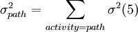
where 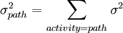 is the summary of all the activities of this pathway. Therefore, if in the equation (5), the activities of the critical path are calculated, the variance of the total time of the project is estimated. The standard deviation of the time is the outcome from the square root of the equation (5).
A very important element of the analysis is the "total duration of the project”. It is a random variable, which can be considered to follow the normal distribution, with average the sum of the expected values and the duration of the activities on the critical path and variance the sum of these variations of these durations. The thoughtfulness behind the project completion time, leads to another level of stochastic analysis of the problem. As is apparent from the above, it is not known for how long the project will last before it is completed, but it is known that the normal distribution with known parameters. In such cases, it is possible to calculate the probability of completing the project within a given time. This calculation is based on the assumption that the total time of the project follows the normal distribution which means that the values of time integration of individual activities is statistically independent, that there is a quite large variety of activities and that the paths which are created, they are also independent.
The planning of a project, whose duration times of the activities are thoughtful, can be divided into two main sections. The first section is calculated using the three estimates for each activity (optimistic, pessimistic, and most-likely time), the expected duration of each of them and the variance or the standard deviation of this duration. Using the expected values, the PERT / CPM method is applied to calculate times ES, EF, LS and LF, to identify the critical path, the ST times and the total expected project completion time. For all of these expected values which are estimated, the corresponding variations and standard deviations can be calculated. If the conditions that were reported are applied, then the total duration of the project, which is a random variable, follows the normal distribution with known mean and deviation. Thus, the second part of the analysis which is related to the finding of the possibility follows in order to complete the task in a given time. This last part is, as the reader perceives, extremely important in the overall analysis of the project, because when there is uncertainty about the durations of activities, it is critical to know the success rate which is associated with the completion of the project within a specific time horizon.
Example
In order the PERT / CTP method to be more understandable, an example is going to be provided.
Exercise
A public service has obtained funds for the design, the installation and the operation of a modern information system. The system is expected to enhance significantly the quality of services to citizens, because it will gradually replace most of the processes which are performed manuscripts. The work is quite complicated and cannot be determined in advance, with reasonable accuracy, the duration of each activity. Thus, taking into account data from other similar projects, estimations were made on the optimists, pessimists and most-likely time of each activity. The example’s data are given in the table below. Time is represented in weeks.

Solution
Initially, it is observed that the development of software (F) is not directly dependent on the supply of material (D), because the opportunity to proceed with the planning work in their own premises, is given to the contractor, even before the receipt of the equipment.
Using the equations (2), (3) and (4), the expected times, the variations and the standard deviations of each activity are calculated. The results of these calculations are given in Table 1.
Table 1

Table 3 shows the PERT/CPM diagram of the project. The virtual activity 11-12 is used for the project to lead to a final node. Then, using the expected times, apply the PERT/CPM method is applied in order the earliest and the latest starting and finishing times of the activities to be estimated. Table 2 shows these estimations.
Table 2
Below follows the timing of the installation of the information system.

Table 3
PERT/CPM diagram of the exercise

As shown, according to the expected times, the critical path is 1-> 2-> 3-> 4-> 5-> 7-> 9->10-> 12 or in other words, the activities A, B, C , F, G, I, J and L. The total expected duration of the project time is the sum of the expected time of the critical activities and it is given by the following equation:

Discussion
There are two rules applying to all the activities of the PERT/CPM diagram which are the followings:
- Rule of calculation the earliest start of an activity (ES):
In a PERT/CPM network, the earliest start time of an activity (ES) that starts from a node, is equal to the latest of the earliest finish times of the activities (EF) that ends up on this node.
- Rule of calculation the latest finish of an activity (LF):
In a PERT/CPM network, the latest finish time of an activity (LF) that ends up on a node, is equal to the lowest of latest start time of an activity (LS) starting from this node
The key questions that can be answered and moreover the general the information which can be acquired by the project manager and by extension, the execution group by constructing the PERT/CPM network are the followings:
- The graphical representation of the activities and in particular, accurate graphical representation of the sequence of prerequisite activities.
- The estimation of the total time that the work will last.
- The identification of the critical activities. In other words, all these activities that must not be delayed because then, the completion of the project will be delayed.
- The identification of non-critical activities. In other words, all these activities which have delay margins without affecting the project.
- For each non-critical activity, the slack time can be detected. In other words, this is the maximum possible margin delay of an activity without charge of the total time of the project.
- The identification of the probability of the project completion within a certain period of time and in particular in cases where the duration times of activities are estimations.
- The ability to monitor the temporal evolution of the project, the allocation of resources and the possibility of revising the program by changing times, identifying new critical activities and reallocating resources.
- The definition of the possibility to reduce the project completion time (crashing), by the determination of the required resources and the activities which need to be fed.
Advantages
- The PERT/CPM diagram defines explicitly and makes visible the dependencies and priorities of the relations between the processes.
- The PERT/CPM helps to identify the critical path.
- The PERT/CPM helps the identification of the early and the late start for each activity.
- The PERT/CPM network provides for, the possible reduction of the duration of the project due to better understanding of the dependencies, leading to improvements on activities and tasks where it is possible.
- The large number of project data can be organized and presented in a diagram for better understanding and easier decision making.
Limitations
- In a PERT/CPM network, there may be hundreds or thousands of activities and individual employment relationships increasing the degree of complexity.
- The network diagrams are large in size and need a large number of pages and special paper sheets.
- The lack of a timeframe for most of the diagrams makes the representation difficult, although colours may help (e.g. specific colour for integrated nodes).
Related Articles
The Gantt chart and the usage nowadays
Gantt Charts as a Tool for Project Management
PRINCE2 - For successful Project Management
Game theory in project management
PRINCE2, A Project Management Methodology
Program evaluation and review technique (PERT)
Scheduling techniques in Project Management
The Critical Path Method (CPM)
References
- ↑ 1.0 1.1 https://en.wikipedia.org/wiki/Program_evaluation_and_review_technique
- ↑ 2.0 2.1 https://en.wikipedia.org/wiki/Critical_path_method
- ↑ https://en.wikipedia.org/wiki/Project_management
- ↑ 4.0 4.1 4.2 4.3 Bruce N. Baker, René L. Eris, Introduction to PERT – CPM, Homewood, III: Irwin, 1964
- ↑ 5.0 5.1 5.2 Moder, J.J., C.R. Phillips and E.W. Davis, Project Management with CPM, PERT and Precedence Diagramming, 3rd ed., Van Nostrand Reinhold, 1983
- ↑ 6.0 6.1 6.2 Richard I. Levin, Charles A. Kirkpatrick, Planning and Control with PERT/CPM, McGraw-Hill Companies: 1966