Decision Tree: Risk & Opportunities

Abstract

Uncertainty is a massive issue in project management and can lead to high cost and disadvantages if not handled correctly. The project manager must therefore be able to make the best decisions based on the information available.
The decision tree is a tool that can aid the project manager to ensure the best outcome of a problem.
It is based on a tree-like model where each branch is a path of decisions and possible events. Each step include the cost and possibility of that event to occur.
By identifying all the possible events and their chance to occur it gives the project manager the ability to calculate the highest probability for each path.
When combining this with the cost of each event the project manager is able to estimate the cost/benefits for each decision.

Method Description

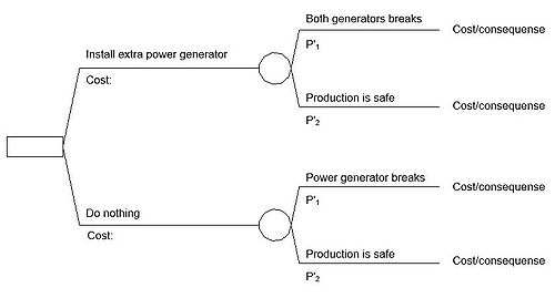
The decision tree is a method to evaluate a decision making process within a project. By using the Bayesion decision analysis the user is able to mitigate the risk and cost of the decision. It is useful when analyzing a process that has a combination of many decisions as the user is able to calculate the effect of each decision. The decision tree is a model with three types of stages:
● A decision node (square)
● A event node (circle)
● A cost/consequence node

At the decision node the project manager has to take an active choice to move on. The event node the effect that can happen from a choice taken. The last type of node is the cost/consequence which is the end result of decisions and events occurring.
Figure 1 shows the basic decision problem situation. It is a medicinal company that is investigating if they should install an extra power generator. If the power generator breaks down they would have to shut down production until it is fixed. A shut down could lead to massive expenses and on the same time investing in an extra power generator is also expensive. First the decision node is whether they should install the power generator or not. Both the decisions leads to an event where there is a chance of two possible outcomes.

Figure 1. Basic decision tree

The theory behind the decision tree is to calculate the average outcome of each decision taken. In short called the Expected cost and can be expressed as this simple equation:
Expected cost = Probability of risk * Impact of the risk
E=P*I

Application of the method

Using the medicinal company's decision problem an example will be presented with the use of a Bayasian decision analysis

Decision analysis - Prior

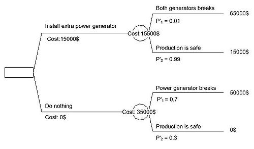
To complete the decision tree information as cost of each stage and the percentage of each event happening must be estimated. For this case the extra power generator cost 15000 $ to install and the aftereffect of the generator breaking down cost 50000 $
If no action is taken there is a 30% chance that the production is safe and 70% it is not.
By installing the generator the production has a 99% to be safe. With really bad luck there is 1% chance that both the generators break down. In the end of each branch the the expenses of each decision and events are summarized. Therefore the expense is 65000$ for the path where both generators break down as the production will get stalled as well.

Figure 2. Decision tree - Prior analysis

The expected cost can now be calculated for each branch as seen with E1 and E2
$E_1 = 0.01\cdot 65000$ + 0.99\cdot 15000$ = 15500$$
$E_2 = 0.70\cdot 50000$=35000$$
The best decision to take is then the minimum of the two expected costs. In this situation it is the path with the extra generator.

Decision analysis - Posterior

If additional information becomes available the decision tree model can be updated.
Given the same case would try to perform a repair on the current power generator.
In the table below are the chance of a repair to be successful. The updated probability can be calculated with the equation in figure 3.

	θ2 Success	θ1 Failure
I1 Repair	0.9	0.1
I2 No repair	0.1	0.9

Figure 3. Equation for posterior probabilities

$P'' = \frac {0.1\cdot 0.7}{0.1\cdot 0.7 + 0.9\cdot 0.3}= 0.2059$
$P'' = \frac {0.9\cdot 0.3}{0.1\cdot 0.7 + 0.9\cdot 0.3}= 0.7941$

References

- ↑ Michael Havbro (2010) Statistics and Probability Theory - In Pursuit of Engineering Decision Support, Publisher : Springer International Publishing.