Earned value management (EVM)
(→Definition of the time-phased budget) |
(→Definition of the time-phased budget) |
||
| Line 74: | Line 74: | ||
|10 | |10 | ||
|} | |} | ||
| − | After creating the Gantt diagram, the BCWS is drawn so that cumulated costs across all scheduled activities are displayed for each time period. More | + | After creating the Gantt diagram, the BCWS is drawn so that cumulated costs across all scheduled activities are displayed for each time period. More specifically, this consists in looking at time axis and the activities axis of the Gantt graph, and checking which activities occur in which period of time. |
<div><ul><li style="display: inline-block;">[[File:Gantt_MR.png|375px|thumb|Figure 2: Gantt diagram (own figure)]]</li><li style="display: inline-block;">[[File:BCWS.png|300px|thumb|Figure 3: BCWS (own figure)]]</li></ul></div> | <div><ul><li style="display: inline-block;">[[File:Gantt_MR.png|375px|thumb|Figure 2: Gantt diagram (own figure)]]</li><li style="display: inline-block;">[[File:BCWS.png|300px|thumb|Figure 3: BCWS (own figure)]]</li></ul></div> | ||
Revision as of 19:44, 27 February 2021
By Martina Rampazzo
Earned value management (EVM) is a methodology for performance measurement which can be applied to individual projects across programs and portfolios [1]. EVM is used in the planning, executing and controlling phases of the PMI Project Management Standard and mainly involves the knowledge areas of scope, time, cost, communication and integration [2]. More specifically, EVM falls into the “project cost management” and “plan schedule and cost management” phases of the PMI Standard of Project Management [3].

Figure 1 shows how earned value management relates to project management phases and the activities which it comprises. While it might appear as a tool mainly related to monitoring and controlling, earned value management methodology brings to the project managers’ attention the importance of performance measurement since the planning phase, with the need for accurate planning and for the realization of a project which is easy to execute and measure.
This article will describe the earned value management methodology applied to projects, with motivations of its relevance, prerequisites for a successful implementation as well as concrete explanations and applications of each of its key metrics. While earned value management is a topic already widely discussed and analyzed in project management from a theoretical point of view, this article will focus on outlining practical real life special cases of projects and how project managers should apply EVM in these cases. Finally, the main limitations of EVM will be discussed thoroughly, including suggestions for project managers on how to face these challenges.
Why project managers should use Earned Value Management?
Earned value management is a tool created by the US Department of Defense in 1967 and used to monitor the Department of Education projects, more specifically the U.S. Large Hadron Collider (LHC) of CERN [4], the world's largest and most powerful particle accelerator [5]. The ability to connect cost and schedule, to identify project performance indicators and express cost and technical performance in an understandable way, led to the diffusion of this tool and to its increased application in the field of project management [6].
Earned value management encompasses earned value analysis, variance analysis and forecasting of future trends. While earned value analysis is limited to define a set of indices to monitor the project’s schedule and cost, earned value management uses this data to also calculate variance and trend analysis, as well as predictions for the future. Therefore, EVM methodology provides a holistic view on the project’s progress and identifies deviations from the plan and budget, allowing project managers to then react to these discrepancies by implementing corrective actions.
The prerequisites for a successful implementation of EVM
There are prerequisites project managers should be aware of in order to implement the methodology in the best possible way. These activities range from planning to monitoring, and consist of:
- Applying the work breakdown structure (WBS - The work breakdown structure in project management) in order to decompose all the projects' activities in control accounts, which are manageable work units with specific scope, cost and schedule. Subsequently, human and material resources have to be allocated to each work package using the organization breakdown structure (OBS)[2];
- Assigning management responsibility to each of the control account[2];
- Planning how to keep track of physical work progress and how to assign budgetary earned value for each activity[2];
- Evaluating the method used to capture expenditures during the life cycle of a project to compare it with the budget[2];
- Implementing change management plans to ensure EVM remains relevant if the project scope changes[7];
- Using an adequate cost collection system to track actual cost and outstanding invoices[7];
- Conducting reporting activities in order to interpret the data obtained and subsequently communicate it to the relevant stakeholders[2].
How to implement EVM
The earned value management methodology comprises four main phases:
- Defining the time-phased budget
- Monitoring time and costs
- Analyzing deviations and defining relevant indices
- Forecasting
Earned value management consists in examining the relationship between three types of curves:
- Budgeted Cost of Work Scheduled (BCWS): the planned and scheduled work - also called PV (planned value)
- Budgeted Cost of Work Performed (BCWP): the actual work performed according to the control account - also called EV (earned value)
- Actual Cost of Work Performed (ACWP): the actual expenditures of the control account up to the period of time in which the curve is analyzed - also called AC (actual cost)
Definition of the time-phased budget
The first step of earned value management is representing the BCWS, also called the baseline of the project, which represents the cumulative cost of the activities for each period of time and therefore aggregates the budgeted cost of all control accounts. The curve can be obtained thanks to the Gantt chart (Gantt Chart in Project Management), which displays the scheduled activities of the project in each unit of time. An example is provided below to clarify this process.
The following set of activities is given, with information on predecessors, scheduled time and budgeted cost.
| Activity | Predecessor | Time | Cost | Monthly cost |
|---|---|---|---|---|
| A | / | 2 | 30 | 15 |
| B | A | 2 | 40 | 20 |
| C | A, B | 1 | 30 | 30 |
| D | B | 4 | 40 | 10 |
After creating the Gantt diagram, the BCWS is drawn so that cumulated costs across all scheduled activities are displayed for each time period. More specifically, this consists in looking at time axis and the activities axis of the Gantt graph, and checking which activities occur in which period of time.
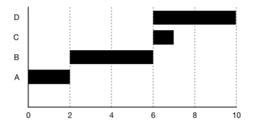 Figure 2: Gantt diagram (own figure)
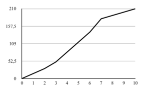 Figure 3: BCWS (own figure)


Monitoring time and costs
Monitoring of costs during the life of a project allows to trace the ACWP, which is the actual cost of work performed. This is extremely relevant as the real costs spent on a project often diverge from the planned ones, as many unforeseen events can occur. Usually actual costs are calculated by checking the actual division of work among manpower and using tools such as cost and time reports, which show how the resources of a team spent their time and the amount of expenditures. [8]
Deviations analysis

BCWS and ACWP alone do not provide any information on the nature of a potential deviation. For example, if ACWP > BCWS, it might be that the project either is inefficient, so actual expenditures are higher than what planned in the budget, or work is being performed earlier compared to the schedule. For this reason it is key to build the third curve, the Budgeted Cost of Work Performed.
The budgeted cost of work performed can be calculated by multiplying the percentage of completion (POC) with the budget at completion (BAC), which is the total budget of the project. The calculation of the BCWP is probably the most complex one since it requires to define the percentage of work actually performed (POC). The different ways to calculate POC will be described further in chapter 4.

A useful way to conduct deviation analysis is to group the 3 metrics into one graph, so that it is easier to compare them. This analysis generates 2n scenarios, where n is the number of parameters being studied. Being that with earned value management, the parameters are time and cost, the possible scenarios are four:
- Project late compared to the schedule and inefficient
- Project late compared to the schedule and efficient
- Project on time/early compared to the schedule and efficient
- Project on time/early compared to the schedule and inefficient
Other than graphically, it is also possible to evaluate time and costs with indicators, both relative and absolute, with the former expressing deviations in percentage, while the latter in monetary units.
Relative indices
Relative indices are cost performance index (CPI) and schedule performance index (SPI). If these indices are greater than one, then the project is efficient and ahead of schedule respectively.

Absolute indices
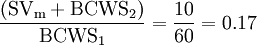
Absolute indices provide the same information of the relative indices but with different formulas, as shown below. In this case, it is preferred to have values larger than 0 for both cost variance (CV) as well as schedule variance expressed in monetary units (SVm).


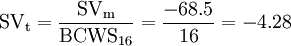
It is important to notice that the schedule variance is expressed in monetary units instead of time units, which would be easier to interpret. This topic was widely discussed from the 1970s, as earned value management originally did not include schedule deviations in time units. According to the article Earned Schedule: An Emerging Enhancement to Earned Value Management by Lipke W.; Henderson K., this situation led over time to project managers using the earned value management methodology primarily to understand costs rather than schedule [[6]]. However, in 2002 the “earned schedule” concept was introduced, a metric which indicates the instant of time in which the BCWS is equal to the BCWP. If these two curves do not match, the projection of the first one onto the second one is the amount of work performed which should be earned according to the schedule (BCWS). The earned schedule is the time from when the project begins up to the projection of this intersection onto the time axis.
In this way, schedule variance can be expressed in time units by subtracting the current period (which in this article will be referred to as Time Now) from the earned schedule. If this value is greater than zero, then it means the project is ahead of schedule. Figure 5 shows the reasoning behind the formula for SVt, where BCWS* corresponds to the Earned Schedule (ES), whereas BCWP* indicates the value at Time Now.

If the trend of the BCWS is constant in the interval of time considered, meaning that the same activity is taking place during the entire time, then the schedule variance in time units can also be expressed with the following formula:
The case in which the BCWS is not constant will be discussed in chapter 6.
Forecasting

By calculating deviation indices, project managers have a picture of the project’s performance in that specific moment. However, before implementing any corrective actions, it is necessary to understand what would be the final arrival point of the project if it continued with the same trend. In fact, identifying, planning, and mobilizing resources to implement corrective actions are time consuming and expensive activities, and may not be necessary if the final performance of the project is within the acceptable range.
The key metrics to forecast future trends are EAC and SAC, which stands for Estimate At Completion and Schedule at Completion. In addition to these metrics, there is also Variance at Completion, which will not be covered in this article (read more about it at [2]). From a graphical point of view, these metrics are obtained by extending the ACWP and the BCWP until the end of the project.
Mathematically, it is important to define which type of potential effects the deviation analysis in step 3 has on the project. The possible scenarios are three.
Scenario 1: The effect of the issue on the project is limited
This is the case of deviations from original planning due to external factors which impacted the project but have ended their effect. For example, this is the case of higher prices for raw materials and therefore higher costs which impact only limited initial activities of the project.

Scenario 2: The effect of the issue on the project is extended
The second category of issues is when the issue impacting the delay and/or the inefficiency of a project is expected to continue in the future and have impacts on the entire project. This is the case that the raw materials transportation was an activity conducted during all the project. There are also other alternatives to this calculation which can be found at Practice Standard for Earned Value Management of Project Management Institute, pg. 21 [2].

Scenario 3: Both types of issues affect the project

Practically speaking, it is possible that the project falls into a grey zone in between the two scenarios and that there are two components of deviations, one for each scenario. In this case, studies from the Department of Management, Economics and Industrial Engineering of Politecnico di Milano suggest the following steps to calculate EAC and SAC[10]. The suggested process is valid if cost and time deviations of scenario 1 are efficiency (Lower cost1 in the formula) and anticipation compared to the schedule (Earlier schedule1 in the formula) respectively. In the opposite case in which scenario 1 deviations are problematic, step 1 and 3 formulas will result having the opposite sign.
- Remove the positive deviation with limited effect and calculate the new ACWP* and BCWP*;

- Calculate CPI* and SPI* and the corresponding EAC* and SAC* with the values obtained in step 1. These are the forecasted values which account only for deviations of scenario 2;
- Calculate EAC and SAC by reintroducing the deviation of scenario 1

To Complete Indexes
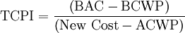
The last step of Earned Value Management consists in defining the SPI and CPI indices the project should have in order to make up for the potential poor performance and reach the desired schedule and cost targets. To evaluate their actual concrete feasibility it is possible to calculate To Complete Schedule Index (TCPI) and To Complete Schedule Index (TSPI):

Project managers should interpret these indices to understand whether it is really feasible to maintain them until the end of the project. With regards to this, a research conducted by the U.S. Department of Defense concluded that once a WBE is over 20% of its completion, CPI and SPI indices should not be increased by 10% [11] because the WBE is considered stable and therefore the final performance will not diverge a lot from the current one.
Percentage of Completion Calculation Methods (POC)
As explained previously, in order to calculate the BCWP, project managers need to estimate the Percentage of Completion, which describes the actual progress of the project. There are many methods to evaluate progress, some objective and others subjective. This article will divide the POC calculation methods according to the division presented in the article Analysis and application of earned value management to the Naval Construction Force [12] and will briefly explain the most relevant limitations of each.
- Discrete effort:
- Milestone Method: assigns a weight to each milestone. Once this is completed, the percentage of completion will increase of the value of the milestone. It suits longer projects and requires more than 2 milestones;
- Fixed Ratio Formula Method: a variation of the previous method which assumes only 2 milestones, one at the beginning of an activity and the second one at the end, with a weighs that may vary but have to add up to 100%. The most common ratios used are 0/100, 50/50 and 25/75;
- Equivalent Unit Method: consists in counting the number of completed units and comparing it to the total units which need to be accomplished. It is applicable only if the activities allow to count physical units, therefore it suits repetitive tasks;
- Percent Complete Method: applies a percentage of completion according to the progress of the activity. It is easier to apply for projects where performance is measurable. In other cases, it is also used as a subjective method where the Control Account manager estimates the percentage of completion according to his experience and knowledge;
- Percent Complete with Milestone Gates Method: a variation of the milestone method which allows to report subjective percentages of completion to the activity until the milestone is reached;
- Earned Standards: determines the percentage of completion according to standards derived from historical data, time and motion studies and other methods. It is challenging to apply one unique standard as every project has its own specific characteristics and is influenced by factors which vary from project to project.
- Apportioned Effort: associates activities which are closely correlated in terms of planning and performance. An example is associating the percentage of completion of the production control to the one of production.
- Level of Effort (LoE): it assumes that the progress of activities is proportional to time. This method should be avoided as it assumes that BCWP is always the same as BCWS. In this way, SV and SPI will always be equal to 0 and 1 respectively and misleading cost variances will be generated.[11]
An important observation on the Percentage of Completion is that there are some methods that are by nature more subjective, like Level of Effort, apportioned effort, percent complete method, and other which are more objective and therefore suit more controlling activities, such as milestone, fixed formula and equivalent unit methods. Project managers should limit the use of subjective methods since their level of accuracy is more questionable and impose a limit on the number of activities controlled with such methods.[11]
Another aspect of the POC is that for those methods which are based on measurable deliverables and outputs (milestones and fixed ratio formula) project managers should reflect upon the duration of the activity and frequency of control in order to keep them as coherent as possible. For example, if an activity is controlled every month, it becomes useless to have milestones every day.[11]
Application of EVM
The following section serves to provide a practical application of the concepts of earned value management explained in the previous chapters. The assumption of this example is that, at the beginning of day 16, controlling and monitoring activities are conducted to evaluate the performance of the project. For clarity of the explanation, the EVM structure previously discussed will be applied in this example step by step.
Defining the time-phased budget (BCWS)
The following table is given, with activities, predecessors, planned duration and costs.
| Activity | Predecessor | Expected Duration | Expected Cost |
|---|---|---|---|
| 1 | / | 5 | 30 |
| 2 | 1 | 8 | 40 |
| 3 | 1 | 10 | 70 |
| 4 | 2 | 4 | 40 |
| 5 | 3 | 10 | 60 |
| 6 | 4, 5 | 12 | 120 |
To calculate the BCWS, it is useful to create the network of the project in order to check which activities should have been completed on day 16 (figure 6, where the critical path has been highlighted in red).

Therefore:

Monitoring time and costs (ACWP)
In this example, it is assumed that it has been monitored ACWP16=90.
Analyzing deviations and defining relevant indices
Under the assumption percentage of completion method is used to calculate BCWP, the Control Account manager provided the following information.
| Activity | Percentage of Completion |
|---|---|
| 1 | 100% |
| 2 | 100% |
| 3 | 25% |
| 4 | 50% |
| 5 | 0% |
| 6 | 0% |
Therefore the BCWP in day 16 is given by:

Relative indices

Absolute indices

The indices show that the project is efficient and late compared to the schedule.
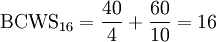
It is also useful to calculate the schedule variance expressed in time units to verify how much days the project is late. In this exercise, the trend of the BCWS in day 16 is constant as no new activity is started, and no activity is finished compared to day 15. In this time period only activities 4 and 5 are occurring, therefore only their respective expected costs and expected durations are considered:
Forecasting
In this example, only scenarios 1 and 2 are applied. The calculations show that issues with an impact on the entire project tend to amplify the effect on the esteems both in positive and in negative.
Scenario 1: The effect of the issue on the project is limited


Scenario 2: The effect of the issue on the project is extended


To Complete Indexes
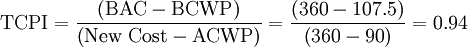


Coherently with the results in step 3), the results of the to complete indices suggest that CPI index can be worsened, while to be able to finish the project in day 37, SPI has to be improved from 0.61 to 1.23, which corresponds to a 101,64% increase. According to criteria of the U.S. Department of Defense explained in chapter 3.5, this is quite improbable.
Special case for schedule variance calculation

When project managers have to deal with monitoring of projects, often real life situations are not as expected from a theoretical point of view. In chapter 3.3 Schedule Variance expressed in time units was presented, under the circumstances that BCWS curve does not change trend in the considered period of time.
However, there are some situations in which this formula is not accurate and may approximate too much the value of SVt. According to studies from the Department of Management, Economics and Industrial Engineering of Politecnico di Milano[13], a way to verify this is to analyze the BCWS in the periods of time which range from the Earned Schedule to Time Now. If the values are the same, then the simplified formula can be applied. Otherwise, the following pragmatic steps are suggested:
- Subtract (or add if SVm is negative) from SVm the values of BCWSperiod for each time period until SVm is equal to 0 (which corresponds to the point in which BCWS and BCWP meet). This will return the interval in which SVt belongs to;
- To determine the decimal values, use the simplified formula using the remaining SVm after having subtracted BCWSperiod in step 1) and as BCWSperiod use the period of time in which SVt falls into.
An example is presented to better understand this process.
In figure 7 it can be seen that BCWS changes trend from ES to Time Now interval of time. Under the hypothesis that SVm = -20, BCWS1 = 60 and BCWS2 = 30, applying formula of chapter 3.3 returns SVt = -0.66. However, looking at the graph it can be seen that it is actually in between 1 and 2. Therefore, applying step 1), SVm is closes to 0 when adding BCWS2 once. This corresponds to SVt being in between 1 and 2. Finally, applying step 2), the decimals are:
Therefore:

This approach is effective as it provides an accurate value for SVt, when the trend of the BCWS is not constant, however it may be challenging to implement for large projects.
Limitations
Based on a collection of articles and books which widely discuss EVM, the following section includes limitations of Earned Value Management methodology project managers should be aware of as well as suggestions on how to face them.
- First of all, the calculation of the BCWP curve is a challenging part of EVM as there is a wide range of methods which can be used with different pros and cons, as discussed in chapter 4 of this article. In fact, project managers have to evaluate the trade off between the inaccuracy of subjective methods and the demanding implementation of discrete methods. Moreover, the choice of the tool for the BCWP calculation is not a controlling but a planning activity and therefore, when planning each activity, it is important to define also what is the best way to control it[12]. Another aspect is that being that POC and BCWP often are approximated values, all the following indices calculated may be imprecise and therefore should always be interpreted according to the context of the project.
- In the forecasting part of EVM, it may also be challenging to understand which type of issue the activity or project is facing and therefore which of the three set of formulas to implement. This is where the prerequisite of project managers having experience and knowledge of project managers helps face this challenge.
- Another problematic aspect concerns the application of formulas for WBEs at the initial stages of completion. Looking at EAC formula in chapter 3.4, the less work is done, the more BCWP will vary from BAC and EAC (€) will diverge from ACWP, the actual work performed. This suggests that forecasting should be carried out with caution especially in the initial phases of the project, as small variations in SPI and CPI indices from 1, can lead to huge variations in the time and cost of the activities, which often do not correspond to reality. An example from the book L'organizzazione dell'impresa by Bartezzaghi Emilio will be taken into consideration. The first assumption is that there are two WBEs, one which is in the early stage (lower than 20% of completion) and another one in the final phases. The second assumption is that these two activities are on time and have the same negative cost variance. According to the formulas, CPI1 is smaller than CPI2 because WBE1 has just begun. The same logic applies to EAC1 and EAC2. This suggests that WBE2 is performing better than WBE1. However, when calculating the TCPI, WBE2 should increase its performance tremendously compared to WBE2 in order to finish the project with the planned total budget. This is due to the fact that WBE2 is nearly finished and therefore it has less time to make up for the cost deviations. For this reason, project managers should always interpret numbers obtained and should impose a limit of variation of esteems of +/- 10% until the project is not stabilized, usually until BCWP=20%*BAC[11].
- Another limitation to EVM with regards to forecasting is that there is always some degree of uncertainty in projects on the different parameters that characterize a project. These parameters are the “activity durations or costs, resource use, the presence of precedence relations or even on the existence of an activity in the project network.” This makes forecasting in EVM a critical step that project managers have to approach carefully. A suggested solution proposed by Vanhoucke Mario in Integrated Project Management Sourcebook' is for project managers to visualize the future trend of these parameters not as a point, but as a dataset, and therefore as a probability distribution. In this way, it is possible to apply simulation models that imitate the progress of parameters as random variables and to understand the overall future trend of the project. More on this can be read in the article RA4: Activity distributions at page 119 [9].
- Another critical point of EVM project managers should be aware of is in case of collaborations with external suppliers. If contracts are based on fixed prices, suppliers are not obliged to reveal their structure of costs and therefore if there are issues with activities based on supply, it is possible to detect possible lateness but not inefficiency. This missing transparency on costs leads to CPI always being 1 and therefore to a lower level of accuracy during the controlling phase.[11]
- Finally, earned value management focuses only on schedule and costs of a project but lacks information on risk and quality, which are key aspects to determine the success of a project. The article Project Management Model: Integrating Earned Schedule, Quality, and Risk in Earned Value Management suggests new indices to combine with traditional earned value management in order to measure quality performance and risk assessment and shows how these new indices increase accuracy for schedule metrics [14].
Annotated Bibliography
This section includes references for further reading on Earned Value Management and its application in project management:
- Project Management Institute, Inc. (2005). Practice Standard for Earned Value Management. Pennsylvania, USA: Project Management Institute, Inc.: this book represents the standards for Earned Value Management methodology, with a strong focus on how it is connected to the project management process and when project managers should apply it. It provides a detailed list of the steps of the methodology as well as special cases project managers might want to consider, for example how the EVM fits different situations depending on the degree of uncertainty and significance of the project as well as the frequency and granularity of the performance measurement. Moreover, the final chapters are dedicated to the prerequisites for application of EVM and guidance on the use of the key metrics.
- Hayes, R. (2001). Analysis and application of earned value management to the Naval Construction Force. California, USA: Naval Postgraduate School (U.S.). Dudley Knox Library: even though the last part of this paper is specific to Naval Construction Force cases, it provides a concise description of EVM and summarizes the several findings of published literature. The first part of the paper also provides information on the origin of the methodology within government and how it evolved throughout the years to become a more user-friendly tool applicable also to private industries, highlighting also the differences with the PERT technique. Finally, it provides a practical application of the methodology to Naval Construction Force project management, not only as a mere application of the formulas but also as an analysis of the planning and execution phases, such as project monitoring and reporting.
- Vanhoucke, M. (2016). Integrated Project Management Sourcebook. Gent, Belgium: Springer: this book deals with the theme of Integrated Project Management and Control, tackling not only earned value management methodology, but also network and resource analysis, scheduling techniques such as PERT and Critical Path Method, schedule risk analysis, buffer management and more. In fact, it comprises of +70 articles which do not only deal with earned value management, but also with other themes that are directly linked to it. In this way, it allows the reader to have a more holistic view and knowledge of baseline scheduling, risk analysis and project control and therefore understand better how to combine EVM with other tools and techniques for project planning, execution and controlling.
- Miguel, A., Madria, W. and Polancos, R. (2019). Project Management Model: Integrating Earned Schedule, Quality, and Risk in Earned Value Management. In: 2019 IEEE 6th International Conference on Industrial Engineering and Applications. De La Salle University Manila, Philippines: Department of Industrial Engineering: this article provides project managers with a new methodology which allows to overcome one of the most important limitations of classic Earned value management, which is the lack of quality and risk performance measurement by proposing a new model which includes risk and quality metrics. The new methodology shows how quality problems affect the cost and schedule of a project and how, from risk indices, preventive actions are taken. These new indices are applied to a sample project in order to validate it from a practical point of view. Finally, this article highlights how, as a consequence, traditional earned value management metrics related to schedule represent a more accurate real time delay.
References
- ↑ Cable, J. H., Ordonez, J. F., Chintalapani, G. and Plaisant, C. (2004). Project portfolio earned value management using Treemaps. Paper presented at PMI® Research Conference: Innovations, London, England. Newtown Square: Project Management Institute. (PMI).
- ↑ 2.0 2.1 2.2 2.3 2.4 2.5 2.6 2.7 2.8 Project Management Institute, Inc. (2005). Practice Standard for Earned Value Management. Pennsylvania, USA: Project Management Institute, Inc. (PMI).
- ↑ Project Management Institute, Inc. (2017). Guide to the Project Management Body of Knowledge (PMBOK® Guide) (6th Edition). Pennsylvania, USA: Project Management Institute, Inc. (PMI).
- ↑ Ferguson J., Kissler K.H. (2002). Earned Value Management. CERN-AS-2002-010
- ↑ CERN.(n.d.).The Large Hadron Collider. Retrieved from https://home.cern/science/accelerators/large-hadron-collider
- ↑ 6.0 6.1 Lipke W.; Henderson K.(2010).Earned Schedule: An Emerging Enhancement to Earned Value Management
- ↑ 7.0 7.1 Lukas J.A. (2008). 2008 AACE INTERNATIONAL TRANSACTIONS. Earned Value Analysis – Why it Doesn't Work
- ↑ Andawei, M. (2014). Project cost monitoring and control: A case of cost/time variance and earned value analysis. IOSR Journal of Engineering (IOSRJEN), Vol. 04, Issue 02, p. 23.
- ↑ 9.0 9.1 9.2 9.3 Vanhoucke, M. (2016). Integrated Project Management Sourcebook. Gent, Belgium: Springer
- ↑ 10.0 10.1 Department of Management, Economics and Industrial Engineering, Politecnico di Milano. (2020). Stime a finire - Scostamenti Contingenti e Strutturali. Milano
- ↑ 11.0 11.1 11.2 11.3 11.4 11.5 Bartezzaghi, E. (2019). L'organizzazione dell'impresa. 4th ed. Milano: Rizzoli ETAS
- ↑ 12.0 12.1 Hayes, R. (2001). Analysis and application of earned value management to the Naval Construction Force. California, USA: Naval Postgraduate School (U.S.). Dudley Knox Library
- ↑ 13.0 13.1 Department of Management, Economics and Industrial Engineering, Politecnico di Milano. (2020). SVtempo - Modalità di calcolo. Milano
- ↑ Miguel, A., Madria, W. and Polancos, R. (2019). Project Management Model: Integrating Earned Schedule, Quality, and Risk in Earned Value Management. In: 2019 IEEE 6th International Conference on Industrial Engineering and Applications. De La Salle University Manila, Philippines: Department of Industrial Engineering